added 220 characters in body
Source Link
whuber
  • 333.5k
  • 63
  • 792
  • 1.3k

I won't prove (B), but intuitively the symmetric positions of the five order statistics used for the 5-letter summary (the boxplot statistics) will produce an estimate symmetrically distributed around the correct parameter, which therefore is unbiased.

A quick simulation shows us how things are shaking out. I chose a sample size of just $n=8,$ because maximum likelihood is most likely to perform poorly for the smallest samples. The 5-letter summary I chose uses the order statistics at positions $1,3,4,6,8,$ which isn't even symmetric  . (theThe median is usually at position $4.5$)$4.5,$ interpreted as the arithmetic mean of the order statistics at positions $4$ and $5$. (For For simplicity, I don't attempt to use quantiles that interpolate among order statistics, so this solution isn't even going to be optimal.)

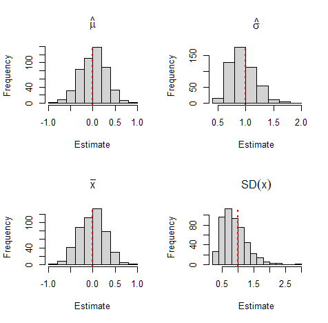
Here are the results of applying this 5-letter summary estimator to $500$ independent samples of a standard Normal distribution (withfor parameters $\mu=0$ and $\sigma=1$$\sigma=1,$ with no loss of generality because the estimator is location and scale covariant), yielding estimates $\hat\mu$ and $\hat\sigma,$ along with the results of applying the usual maximum likelihood estimates $\bar x$ (the mean) and $\operatorname{SD}(x)$ (computed as the root mean squared deviation from the mean, not with any bias correction).
I won't prove (B), but intuitively the symmetric positions of the five order statistics used for the 5-letter summary (the boxplot statistics) will produce an estimate symmetrically distributed around the correct parameter.

A quick simulation shows us how things are shaking out. I chose a sample size of just $n=8,$ because maximum likelihood is most likely to perform poorly for the smallest samples. The 5-letter summary I chose uses the order statistics at positions $1,3,4,6,8,$ which isn't even symmetric  (the median is at position $4.5$). (For simplicity, I don't attempt to use quantiles that interpolate among order statistics, so this solution isn't even going to be optimal.)

Here are the results of applying this estimator to $500$ independent samples of a standard Normal distribution (with parameters $\mu=0$ and $\sigma=1$), yielding estimates $\hat\mu$ and $\hat\sigma,$ along with the results of applying the usual maximum likelihood estimates $\bar x$ (the mean) and $\operatorname{SD}(x)$ (computed as the root mean squared deviation from the mean, not with any bias correction).

I won't prove (B), but intuitively the symmetric positions of the five order statistics used for the 5-letter summary (the boxplot statistics) will produce an estimate symmetrically distributed around the correct parameter, which therefore is unbiased.

A quick simulation shows us how things are shaking out. I chose a sample size of just $n=8,$ because maximum likelihood is most likely to perform poorly for the smallest samples. The 5-letter summary I chose uses the order statistics at positions $1,3,4,6,8,$ which isn't even symmetric. (The median is usually at position $4.5,$ interpreted as the arithmetic mean of the order statistics at positions $4$ and $5$. For simplicity, I don't attempt to use quantiles that interpolate among order statistics, so this solution isn't even going to be optimal.)

Here are the results of applying this 5-letter summary estimator to $500$ independent samples of a standard Normal distribution (for parameters $\mu=0$ and $\sigma=1,$ with no loss of generality because the estimator is location and scale covariant), yielding estimates $\hat\mu$ and $\hat\sigma,$ along with the results of applying the usual maximum likelihood estimates $\bar x$ (the mean) and $\operatorname{SD}(x)$ (computed as the root mean squared deviation from the mean, not with any bias correction).

added 72 characters in body
Source Link
whuber
  • 333.5k
  • 63
  • 792
  • 1.3k
#
# Negative log likelihood.
#
Lambda <- function(theta, values, orders) {
  mu <- theta[1]
  log.sigma <- theta[2]
  sigma <- exp(log.sigmatheta[2])
  f <- dnorm(values, mu, sigma, log = TRUE)
  F <- log(diff(pnorm(c(-Inf, values, Inf), mu, sigma)))
  -(sum(f) + sum(F * (diff(c(0, orders, n+1))-1)))
}
#
# A simulation study.
#
n <- 8
q <- c(`X-` = 0, `H-` = 1/4, M = 1/2, `H+` = 3/4, `X+` = 1)
orders <- round(quantile(seq_len(n), q))
 
mu <- 0
0; sigma <- 1
set.seed(17)
sim <- replicate(5e2, {
  x <- rnorm(n, mu, sigma)  # The full dataset
  nletter <- quantile(x, q) # Its 5-letter summary
  #
  # Compute the estimate.
  #
  theta.start <- c(mu = mean(range(nletter)), 
                   log.sigma = log(diff(range(nletter)) / 6))
  fit <- nlm(Lambda, theta.start, values = nletter, orders = orders) 
  if (fit$code > 2) warning("nlm did not succeed.")
  theta.hat <- setNames(fit$estimatefit$code > 2) warning("nlm did not succeed.")
  theta.hat <- setNames(fit$estimate, names(theta.start))
  c(theta.hat, xbar = mean(x), sd = mean((x - mean(x))^2))
})
sim[2, ] <- exp(sim[2, ]) # (The log of sigma was estimated.)
rownames(sim) <- c("mu.hat", "sigma.hat", "x.bar", "SD")
#
# Negative log likelihood.
#
Lambda <- function(theta, values, orders) {
  mu <- theta[1]
  log.sigma <- theta[2]
  sigma <- exp(log.sigma)
  f <- dnorm(values, mu, sigma, log = TRUE)
  F <- log(diff(pnorm(c(-Inf, values, Inf), mu, sigma)))
  -(sum(f) + sum(F * (diff(c(0, orders, n+1))-1)))
}
#
# A simulation study.
#
n <- 8
q <- c(`X-` = 0, `H-` = 1/4, M = 1/2, `H+` = 3/4, `X+` = 1)
orders <- round(quantile(seq_len(n), q))
 
mu <- 0
sigma <- 1
set.seed(17)
sim <- replicate(5e2, {
  x <- rnorm(n, mu, sigma)
  nletter <- quantile(x, q)
  #
  # Compute the estimate.
  #
  theta.start <- c(mu = mean(range(nletter)), log.sigma = log(diff(range(nletter)) / 6))
  fit <- nlm(Lambda, theta.start, values = nletter, orders = orders) 
  if (fit$code > 2) warning("nlm did not succeed.")
  theta.hat <- setNames(fit$estimate, names(theta.start))
  c(theta.hat, xbar = mean(x), sd = mean((x - mean(x))^2))
})
sim[2, ] <- exp(sim[2, ])
rownames(sim) <- c("mu.hat", "sigma.hat", "x.bar", "SD")
#
# Negative log likelihood.
#
Lambda <- function(theta, values, orders) {
  mu <- theta[1]
  sigma <- exp(theta[2])
  f <- dnorm(values, mu, sigma, log = TRUE)
  F <- log(diff(pnorm(c(-Inf, values, Inf), mu, sigma)))
  -(sum(f) + sum(F * (diff(c(0, orders, n+1))-1)))
}
#
# A simulation study.
#
n <- 8
q <- c(`X-` = 0, `H-` = 1/4, M = 1/2, `H+` = 3/4, `X+` = 1)
orders <- round(quantile(seq_len(n), q))
mu <- 0; sigma <- 1
set.seed(17)
sim <- replicate(5e2, {
  x <- rnorm(n, mu, sigma)  # The full dataset
  nletter <- quantile(x, q) # Its 5-letter summary
  #
  # Compute the estimate.
  #
  theta.start <- c(mu = mean(range(nletter)), 
                   log.sigma = log(diff(range(nletter)) / 6))
  fit <- nlm(Lambda, theta.start, values = nletter, orders = orders) 
  if (fit$code > 2) warning("nlm did not succeed.")
  theta.hat <- setNames(fit$estimate, names(theta.start))
  c(theta.hat, xbar = mean(x), sd = mean((x - mean(x))^2))
})
sim[2, ] <- exp(sim[2, ]) # (The log of sigma was estimated.)
rownames(sim) <- c("mu.hat", "sigma.hat", "x.bar", "SD")
Source Link
whuber
  • 333.5k
  • 63
  • 792
  • 1.3k

The maximum likelihood solution I posted long ago at Estimating a normal distribution from three order statistics works well. The only questions concern (A) how well and (B) whether its estimate of the mean is unbiased.

There are some surprises.

I won't prove (B), but intuitively the symmetric positions of the five order statistics used for the 5-letter summary (the boxplot statistics) will produce an estimate symmetrically distributed around the correct parameter.

This leaves (A). Let's compare the maximum likelihood estimates of the parameters $\mu$ and $\sigma$ to those that would be obtained using all the data.

A quick simulation shows us how things are shaking out. I chose a sample size of just $n=8,$ because maximum likelihood is most likely to perform poorly for the smallest samples. The 5-letter summary I chose uses the order statistics at positions $1,3,4,6,8,$ which isn't even symmetric (the median is at position $4.5$). (For simplicity, I don't attempt to use quantiles that interpolate among order statistics, so this solution isn't even going to be optimal.)

Here are the results of applying this estimator to $500$ independent samples of a standard Normal distribution (with parameters $\mu=0$ and $\sigma=1$), yielding estimates $\hat\mu$ and $\hat\sigma,$ along with the results of applying the usual maximum likelihood estimates $\bar x$ (the mean) and $\operatorname{SD}(x)$ (computed as the root mean squared deviation from the mean, not with any bias correction).

enter image description here

The surprises are

  1. The distribution of $\hat \mu$ scarcely differs from that of $\bar x.$ Compare the histograms in the left column and see the summary below.

  2. The distribution of $\hat\sigma$ is narrower, less skewed, and less biased than the distribution of $\operatorname{SD}(x)$! (Compare the histograms in the right column and notice the slightly wider range of the x-axis at the bottom.)

  3. Because I used asymmetric order statistics, the estimate of the mean is (slightly) biased (high in this case). (To obtain an unbiased estimate, one could take two estimates where the median is considered as either at position $4$ or position $5$ and average the two estimates.)

Here are the averages and standard errors from these $500$ samples:

             Mean     SE
mu.hat     0.0046 0.0130
x.bar     -0.0200 0.0130
sigma.hat  0.9500 0.0098
SD         0.8900 0.0180

To demonstrate the lack of bias in $\hat\mu$ when the order statistics are symmetric (that is, they are at positions $1,$ $k,$ $(n+1)/2$, $n+1-k,$ and $n$ -- and therefore $n$ must be odd), I re-ran the simulation for a sample size of $n=9$ (for order statistics $1,3,5,7,$ and $9$) and created $5000$ samples for greater precision. The histograms are about the same as before, but here are the summary statistics:

            Mean     SE
mu.hat    0.0062 0.0049
x.bar     0.0071 0.0048
sigma.hat 0.9100 0.0034
SD        0.8900 0.0063

Now neither of the estimates of the mean (first two rows) differs significantly from zero (both are well within two SEs of zero) and $\hat\sigma$ is still superior to $\operatorname{SD}(x),$ although not by as much as before.

Finally, here is a summary for $n=79,$ again with $5000$ samples (using order statistics $1,20,40,60,$ and $79$).

                Mean      SE
mu.hat     0.000160 0.00168
x.bar     -0.000624 0.00160
sigma.hat  0.978000 0.00135
SD         0.988000 0.00226

TANSTAAFL, and reality intrudes: $\bar x$ must be superior to $\hat\mu,$ and so it is, as evidenced by its slightly smaller standard error. But $\hat\mu$ remains unbiased. Also, there is no detectable difference now between $\hat\sigma$ and $\operatorname{SD}(x),$ both of which are closely approximating $\sigma = 1.$

Because the performance of $\hat\mu$ is practically the same as that of $\bar x,$ which is a minimum variance unbiased estimator based on all the data, in most applications it would be pointless to try to improve on $\hat\mu.$

It would still be interesting to compare these estimators to the linear-combination-of-order-statistics estimators proposed in other answers, because those are attractive approaches and can admit simpler computation.


Here are details of the simulations (set up to perform the first one). At the end, the four estimates are contained in the four rows of sim. Plotting their histograms is routine and omitted for brevity.

#
# Negative log likelihood.
#
Lambda <- function(theta, values, orders) {
  mu <- theta[1]
  log.sigma <- theta[2]
  sigma <- exp(log.sigma)
  f <- dnorm(values, mu, sigma, log = TRUE)
  F <- log(diff(pnorm(c(-Inf, values, Inf), mu, sigma)))
  -(sum(f) + sum(F * (diff(c(0, orders, n+1))-1)))
}
#
# A simulation study.
#
n <- 8
q <- c(`X-` = 0, `H-` = 1/4, M = 1/2, `H+` = 3/4, `X+` = 1)
orders <- round(quantile(seq_len(n), q))

mu <- 0
sigma <- 1
set.seed(17)
sim <- replicate(5e2, {
  x <- rnorm(n, mu, sigma)
  nletter <- quantile(x, q)
  #
  # Compute the estimate.
  #
  theta.start <- c(mu = mean(range(nletter)), log.sigma = log(diff(range(nletter)) / 6))
  fit <- nlm(Lambda, theta.start, values = nletter, orders = orders) 
  if (fit$code > 2) warning("nlm did not succeed.")
  theta.hat <- setNames(fit$estimate, names(theta.start))
  c(theta.hat, xbar = mean(x), sd = mean((x - mean(x))^2))
})
sim[2, ] <- exp(sim[2, ])
rownames(sim) <- c("mu.hat", "sigma.hat", "x.bar", "SD")