Revisions to Normalize the ratio predictor variable by logit or not?

Commonmark migration

Source Link

edited Jun 11, 2020 at 14:32

1

I have a Poisson GLM model

m1 <- glm(count ~ x, data = data, family = "quasipoisson")

The predictor variable x is a cumulative sum of ratios, i.e. real numbers between 0 and 1. (Not important for this question, but if you are interested why the sum is needed, it is because it is a transformation of a simpler but recursive model).

##Is it desirable to normalize the predictor variable by logit?

Is it desirable to normalize the predictor variable by logit?

i.e. instead of using cumulative sum of ratios, use cumulative sum of logit of the ratios (x2)?

m2 <- glm(count ~ x2, data = data, family = "quasipoisson")

I tried to look at the q-q plots (plot(model)) but they seem to be the same. However I tried to do another plot which is not present in the plot(model) output - I don't know if it's actually important or not. So see comparison of the two models on this plot:

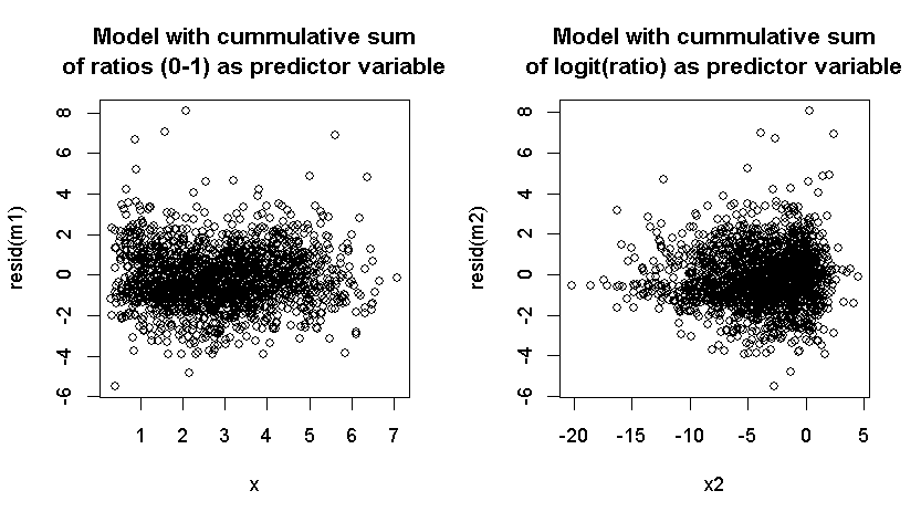
enter image description here

Is this plot actually important for this decision? Does the second plot actually show heteroscedasticity? If yes, then is the original model (without transformation) possibly better according to these plots?

I have a Poisson GLM model

m1 <- glm(count ~ x, data = data, family = "quasipoisson")

The predictor variable x is a cumulative sum of ratios, i.e. real numbers between 0 and 1. (Not important for this question, but if you are interested why the sum is needed, it is because it is a transformation of a simpler but recursive model).

##Is it desirable to normalize the predictor variable by logit?

i.e. instead of using cumulative sum of ratios, use cumulative sum of logit of the ratios (x2)?

m2 <- glm(count ~ x2, data = data, family = "quasipoisson")

I tried to look at the q-q plots (plot(model)) but they seem to be the same. However I tried to do another plot which is not present in the plot(model) output - I don't know if it's actually important or not. So see comparison of the two models on this plot:

enter image description here

Is this plot actually important for this decision? Does the second plot actually show heteroscedasticity? If yes, then is the original model (without transformation) possibly better according to these plots?

I have a Poisson GLM model

m1 <- glm(count ~ x, data = data, family = "quasipoisson")

The predictor variable x is a cumulative sum of ratios, i.e. real numbers between 0 and 1. (Not important for this question, but if you are interested why the sum is needed, it is because it is a transformation of a simpler but recursive model).

Is it desirable to normalize the predictor variable by logit?

i.e. instead of using cumulative sum of ratios, use cumulative sum of logit of the ratios (x2)?

m2 <- glm(count ~ x2, data = data, family = "quasipoisson")

I tried to look at the q-q plots (plot(model)) but they seem to be the same. However I tried to do another plot which is not present in the plot(model) output - I don't know if it's actually important or not. So see comparison of the two models on this plot:

enter image description here

Is this plot actually important for this decision? Does the second plot actually show heteroscedasticity? If yes, then is the original model (without transformation) possibly better according to these plots?

replaced http://stats.stackexchange.com/ with https://stats.stackexchange.com/

Source Link

edited Apr 13, 2017 at 12:44

Community Bot

1

I have a Poisson GLM model

m1 <- glm(count ~ x, data = data, family = "quasipoisson")

The predictor variable x is a cumulative sum of ratios, i.e. real numbers between 0 and 1. (Not important for this question, but if you are interested why the sum is needed, it is because it is a transformation of a simpler but recursive model of a simpler but recursive model).

##Is it desirable to normalize the predictor variable by logit?

i.e. instead of using cumulative sum of ratios, use cumulative sum of logit of the ratios (x2)?

m2 <- glm(count ~ x2, data = data, family = "quasipoisson")

I tried to look at the q-q plots (plot(model)) but they seem to be the same. However I tried to do another plot which is not present in the plot(model) output - I don't know if it's actually important or not. So see comparison of the two models on this plot:

enter image description here

Is this plot actually important for this decision? Does the second plot actually show heteroscedasticity? If yes, then is the original model (without transformation) possibly better according to these plots?

I have a Poisson GLM model

m1 <- glm(count ~ x, data = data, family = "quasipoisson")

The predictor variable x is a cumulative sum of ratios, i.e. real numbers between 0 and 1. (Not important for this question, but if you are interested why the sum is needed, it is because it is a transformation of a simpler but recursive model).

##Is it desirable to normalize the predictor variable by logit?

i.e. instead of using cumulative sum of ratios, use cumulative sum of logit of the ratios (x2)?

m2 <- glm(count ~ x2, data = data, family = "quasipoisson")

I tried to look at the q-q plots (plot(model)) but they seem to be the same. However I tried to do another plot which is not present in the plot(model) output - I don't know if it's actually important or not. So see comparison of the two models on this plot:

enter image description here

Is this plot actually important for this decision? Does the second plot actually show heteroscedasticity? If yes, then is the original model (without transformation) possibly better according to these plots?

I have a Poisson GLM model

m1 <- glm(count ~ x, data = data, family = "quasipoisson")

The predictor variable x is a cumulative sum of ratios, i.e. real numbers between 0 and 1. (Not important for this question, but if you are interested why the sum is needed, it is because it is a transformation of a simpler but recursive model).

##Is it desirable to normalize the predictor variable by logit?

i.e. instead of using cumulative sum of ratios, use cumulative sum of logit of the ratios (x2)?

m2 <- glm(count ~ x2, data = data, family = "quasipoisson")

I tried to look at the q-q plots (plot(model)) but they seem to be the same. However I tried to do another plot which is not present in the plot(model) output - I don't know if it's actually important or not. So see comparison of the two models on this plot:

enter image description here

Is this plot actually important for this decision? Does the second plot actually show heteroscedasticity? If yes, then is the original model (without transformation) possibly better according to these plots?

added 1 characters in body

Source Link

edited Aug 25, 2013 at 11:30

Nick Cox

59.5k
8
136
212

I have a poissonPoisson GLM model

m1 <- glm(count ~ x, data = data, family = "quasipoisson")

The predictor variable x is a cummulativecumulative sum of ratios, i.e. real numbers between 0 and 1. (Not important for this question, but if you are interested why the sum is needed, it is because it is a transformation of a simpler but recursive model).

##Is it desirable to normalize the predictor variable by logit?

Ii.e. instead of using cummulativecumulative sum of ratios, use cummulativecumulative sum of logit of the ratios (x2)?

m2 <- glm(count ~ x2, data = data, family = "quasipoisson")

I tried to look at the q-q plots (plot(model)) but they seem to be the same. However I tried to do another plot which is not present in the plot(model) output - I don't know if it's actually important or not. So see comparison of the two models on this plot:

enter image description here

Is this plot actually important for this decision? Does the second plot actually show heteroscedasticity? If yes, then is the original model (without transformation) possibly better according to these plots?

I have a poisson GLM model

m1 <- glm(count ~ x, data = data, family = "quasipoisson")

The predictor variable x is a cummulative sum of ratios, i.e. real numbers between 0 and 1. (Not important for this question, but if you are interested why the sum is needed, it is because it is transformation of simpler but recursive model).

##Is it desirable to normalize the predictor variable by logit?

I.e. instead of using cummulative sum of ratios, use cummulative sum of logit of the ratios (x2)?

m2 <- glm(count ~ x2, data = data, family = "quasipoisson")

I tried to look at the q-q plots (plot(model)) but they seem to be the same. However I tried to do another plot which is not present in the plot(model) output - I don't know if it's actually important or not. So see comparison of the two models on this plot:

enter image description here

Is this plot actually important for this decision? Does the second plot actually show heteroscedasticity? If yes, then is the original model (without transformation) possibly better according to these plots?

I have a Poisson GLM model

m1 <- glm(count ~ x, data = data, family = "quasipoisson")

The predictor variable x is a cumulative sum of ratios, i.e. real numbers between 0 and 1. (Not important for this question, but if you are interested why the sum is needed, it is because it is a transformation of a simpler but recursive model).

##Is it desirable to normalize the predictor variable by logit?

i.e. instead of using cumulative sum of ratios, use cumulative sum of logit of the ratios (x2)?

m2 <- glm(count ~ x2, data = data, family = "quasipoisson")

I tried to look at the q-q plots (plot(model)) but they seem to be the same. However I tried to do another plot which is not present in the plot(model) output - I don't know if it's actually important or not. So see comparison of the two models on this plot:

enter image description here

Is this plot actually important for this decision? Does the second plot actually show heteroscedasticity? If yes, then is the original model (without transformation) possibly better according to these plots?

Source Link

asked Aug 25, 2013 at 10:58

Tomas

6.2k
14
62
106

Loading

Stack Exchange Network

Return to Question

Is it desirable to normalize the predictor variable by logit?

Is it desirable to normalize the predictor variable by logit?