Minor addition
Source Link
QuantIbex
  • 4.1k
  • 1
  • 31
  • 44

Assuming that the decisions of invited persons to come to the wedding are independent, the number of guests that will come to the wedding can be modeled as the sum of Bernoulli random variables that have not necessarily identical probabilities of success. This corresponds to the Poisson binomial distribution.

Let $X$ be a random variable corresponding to the total number of persons that will come to your wedding out of $N$ invited persons. The expected number of participants is indeed the sum of individual ''show-up'' probabilities $p_i$, that is $$ E(X) = \sum_{i = 1}^N p_i . $$ The derivation of confidence intervals isn't straightforward given the form of the probability mass function. However, they are easy to approximate with Monte Carlo simulations.

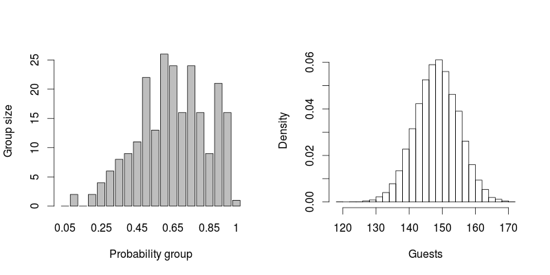
The following figure shows an example of the distribution of the number of participants to the wedding based on 10000 simulated scenarios (right) using some fake show-up probabilities for the 230 invited persons (left). The R code used to run this simulation is shown below; it provides approximations of confidence intervals.
enter image description here

## Parameters
N      <- 230    # Number of potential guests
nb.sim <- 10000  # Number of simulations

## Create example of groups of guests with same show-up probability
set.seed(345)
tmp    <- hist(rbeta(N, 3, 2), breaks = seq(0, 1, length.out = 21))
p      <- tmp$breaks[-1]    # Group show-up probabilities
n      <- tmp$counts        # Number of person per group

## Generate number of guests by group
guest.mat <- matrix(NA, nrow = nb.sim, ncol = length(p))
for (j in 1:length(p)) {
    guest.mat[, j] <- rbinom(nb.sim, n[j], p[j])
}

## Number of guest per scenario
nb.guests <- apply(guest.mat, 1, sum)

## Result summary
par(mfrow = c(1, 2))
barplot(n, names.arg = p, xlab = "Probability group", ylab = "Group size")
hist(nb.guests, breaks = 21, probability =  TRUE, main = "", xlab = "Guests")
par(mfrow = c(1, 1))

## Theoretical mean and variance
c(sum(n * p), sum(n * p * (1-p)))
#[1] 148.8500  43.8475

## Sample mean and variance
c(mean(nb.guests), var(nb.guests))
#[1] 148.86270  43.23657

## Sample quantiles
quantile(nb.guests, probs = c(0.01, 0.05, 0.5, 0.95, 0.99))
#1%     5%    50%    95%    99% 
#133.99 138.00 149.00 160.00 164.00 

Assuming that the decisions of invited persons to come to the wedding are independent, the number of guests that will come to the wedding can be modeled as the sum of Bernoulli random variables that have not necessarily identical probabilities of success. This corresponds to the Poisson binomial distribution.

Let $X$ be a random variable corresponding to the total number of persons that will come to your wedding out of $N$ invited persons. The expected number of participants is indeed the sum of individual ''show-up'' probabilities $p_i$, that is $$ E(X) = \sum_{i = 1}^N p_i . $$ The derivation of confidence intervals isn't straightforward given the form of the probability mass function. However, they are easy to approximate with simulations.

The following figure shows an example of the distribution of the number of participants to the wedding based on 10000 simulated scenarios (right) using some fake show-up probabilities for the 230 invited persons (left). The R code used to run this simulation is shown below; it provides approximations of confidence intervals.

enter image description here

## Parameters
N      <- 230    # Number of potential guests
nb.sim <- 10000  # Number of simulations

## Create example of groups of guests with same show-up probability
set.seed(345)
tmp    <- hist(rbeta(N, 3, 2), breaks = seq(0, 1, length.out = 21))
p      <- tmp$breaks[-1]    # Group show-up probabilities
n      <- tmp$counts        # Number of person per group

## Generate number of guests by group
guest.mat <- matrix(NA, nrow = nb.sim, ncol = length(p))
for (j in 1:length(p)) {
    guest.mat[, j] <- rbinom(nb.sim, n[j], p[j])
}

## Number of guest per scenario
nb.guests <- apply(guest.mat, 1, sum)

## Result summary
par(mfrow = c(1, 2))
barplot(n, names.arg = p, xlab = "Probability group", ylab = "Group size")
hist(nb.guests, breaks = 21, probability =  TRUE, main = "", xlab = "Guests")
par(mfrow = c(1, 1))

## Theoretical mean and variance
c(sum(n * p), sum(n * p * (1-p)))
#[1] 148.8500  43.8475

## Sample mean and variance
c(mean(nb.guests), var(nb.guests))
#[1] 148.86270  43.23657

## Sample quantiles
quantile(nb.guests, probs = c(0.01, 0.05, 0.5, 0.95, 0.99))
#1%     5%    50%    95%    99% 
#133.99 138.00 149.00 160.00 164.00 

Assuming that the decisions of invited persons to come to the wedding are independent, the number of guests that will come to the wedding can be modeled as the sum of Bernoulli random variables that have not necessarily identical probabilities of success. This corresponds to the Poisson binomial distribution.

Let $X$ be a random variable corresponding to the total number of persons that will come to your wedding out of $N$ invited persons. The expected number of participants is indeed the sum of individual ''show-up'' probabilities $p_i$, that is $$ E(X) = \sum_{i = 1}^N p_i . $$ The derivation of confidence intervals isn't straightforward given the form of the probability mass function. However, they are easy to approximate with Monte Carlo simulations.

The following figure shows an example of the distribution of the number of participants to the wedding based on 10000 simulated scenarios (right) using some fake show-up probabilities for the 230 invited persons (left). The R code used to run this simulation is shown below; it provides approximations of confidence intervals.

enter image description here

## Parameters
N      <- 230    # Number of potential guests
nb.sim <- 10000  # Number of simulations

## Create example of groups of guests with same show-up probability
set.seed(345)
tmp    <- hist(rbeta(N, 3, 2), breaks = seq(0, 1, length.out = 21))
p      <- tmp$breaks[-1]    # Group show-up probabilities
n      <- tmp$counts        # Number of person per group

## Generate number of guests by group
guest.mat <- matrix(NA, nrow = nb.sim, ncol = length(p))
for (j in 1:length(p)) {
    guest.mat[, j] <- rbinom(nb.sim, n[j], p[j])
}

## Number of guest per scenario
nb.guests <- apply(guest.mat, 1, sum)

## Result summary
par(mfrow = c(1, 2))
barplot(n, names.arg = p, xlab = "Probability group", ylab = "Group size")
hist(nb.guests, breaks = 21, probability =  TRUE, main = "", xlab = "Guests")
par(mfrow = c(1, 1))

## Theoretical mean and variance
c(sum(n * p), sum(n * p * (1-p)))
#[1] 148.8500  43.8475

## Sample mean and variance
c(mean(nb.guests), var(nb.guests))
#[1] 148.86270  43.23657

## Sample quantiles
quantile(nb.guests, probs = c(0.01, 0.05, 0.5, 0.95, 0.99))
#1%     5%    50%    95%    99% 
#133.99 138.00 149.00 160.00 164.00 
Corrected typos
Source Link
QuantIbex
  • 4.1k
  • 1
  • 31
  • 44

Assuming that the decisions of invited persons to come to the wedding are independent, the number of guests that will come to the wedding can be modeled as the sum of Bernoulli random variables that have not necessarily identical probabilities of success. This corresponds to the Poisson binomial distribution.

Let $X$ be a random variable corresponding to the total number of persons that will come to ouryour wedding out of $N$ invited persons. The expected number of participants is indeed the sum of individual "show''show-up"up'' probabilities $p_i$, that is $$ E(X) = \sum_{i = 1}^N p_i . $$ The derivation of confidence intervals isn't straightforward given the form of the form of the probability mass function. However, they are easy to approximate with simulations.

The following figure shows an example of the distribution of the number of participants to the wedding based on 10000 simulated scenarios (right) using some fake show-up probabilities for the 230 invited persons (left). The R code used to run this simulation is shown below and contains approximationbelow; it provides approximations of confidence intervals.

enter image description here

## Parameters
N      <- 230    # Number of potential guests
nb.sim <- 10000  # Number of simulations

## Create example of groups of guests with same show-up probability
set.seed(345)
tmp    <- hist(rbeta(N, 3, 2), breaks = seq(0, 1, length.out = 21))
p      <- tmp$breaks[-1]    # Group show-up probabilities
n      <- tmp$counts        # Number of person per group

## Generate number of guests by group
guest.mat <- matrix(NA, nrow = nb.sim, ncol = length(p))
for (j in 1:length(p)) {
    guest.mat[, j] <- rbinom(nb.sim, n[j], p[j])
}

## Number of guest per scenario
nb.guests <- apply(guest.mat, 1, sum)

## Result summary
par(mfrow = c(1, 2))
barplot(n, names.arg = p, xlab = "Probability group", ylab = "Group size")
hist(nb.guests, breaks = 21, probability =  TRUE, main = "", xlab = "Guests")
par(mfrow = c(1, 1))

## Theoretical mean and variance
c(sum(n * p), sum(n * p * (1-p)))
#[1] 148.8500  43.8475

## Sample mean and variance
c(mean(nb.guests), var(nb.guests))
#[1] 148.86270  43.23657

## Sample quantiles
quantile(nb.guests, probs = c(0.01, 0.05, 0.5, 0.95, 0.99))
#1%     5%    50%    95%    99% 
#133.99 138.00 149.00 160.00 164.00 

Assuming that the decisions of invited persons to come to the wedding are independent, the number of guests that will come to the wedding can be modeled as the sum of Bernoulli random variables that have not necessarily identical probabilities of success. This corresponds to the Poisson binomial distribution.

Let $X$ be a random variable corresponding to the total number of persons that will come to our wedding out of $N$ invited persons. The expected number of participants is indeed the sum of individual "show-up" probabilities $p_i$, that is $$ E(X) = \sum_{i = 1}^N p_i . $$ The derivation of confidence intervals isn't straightforward given the form of the form of the probability mass function. However, they are easy to approximate with simulations.

The following figure shows an example of the distribution of the number of participants to the wedding based on 10000 simulated scenarios (right) using some fake show-up probabilities for the 230 invited persons (left). The R code used to run this simulation is shown below and contains approximation of confidence intervals.

enter image description here

## Parameters
N      <- 230    # Number of potential guests
nb.sim <- 10000  # Number of simulations

## Create example of groups of guests with same show-up probability
set.seed(345)
tmp    <- hist(rbeta(N, 3, 2), breaks = seq(0, 1, length.out = 21))
p      <- tmp$breaks[-1]    # Group show-up probabilities
n      <- tmp$counts        # Number of person per group

## Generate number of guests by group
guest.mat <- matrix(NA, nrow = nb.sim, ncol = length(p))
for (j in 1:length(p)) {
    guest.mat[, j] <- rbinom(nb.sim, n[j], p[j])
}

## Number of guest per scenario
nb.guests <- apply(guest.mat, 1, sum)

## Result summary
par(mfrow = c(1, 2))
barplot(n, names.arg = p, xlab = "Probability group", ylab = "Group size")
hist(nb.guests, breaks = 21, probability =  TRUE, main = "", xlab = "Guests")
par(mfrow = c(1, 1))

## Theoretical mean and variance
c(sum(n * p), sum(n * p * (1-p)))
#[1] 148.8500  43.8475

## Sample mean and variance
c(mean(nb.guests), var(nb.guests))
#[1] 148.86270  43.23657

## Sample quantiles
quantile(nb.guests, probs = c(0.01, 0.05, 0.5, 0.95, 0.99))
#1%     5%    50%    95%    99% 
#133.99 138.00 149.00 160.00 164.00 

Assuming that the decisions of invited persons to come to the wedding are independent, the number of guests that will come to the wedding can be modeled as the sum of Bernoulli random variables that have not necessarily identical probabilities of success. This corresponds to the Poisson binomial distribution.

Let $X$ be a random variable corresponding to the total number of persons that will come to your wedding out of $N$ invited persons. The expected number of participants is indeed the sum of individual ''show-up'' probabilities $p_i$, that is $$ E(X) = \sum_{i = 1}^N p_i . $$ The derivation of confidence intervals isn't straightforward given the form of the probability mass function. However, they are easy to approximate with simulations.

The following figure shows an example of the distribution of the number of participants to the wedding based on 10000 simulated scenarios (right) using some fake show-up probabilities for the 230 invited persons (left). The R code used to run this simulation is shown below; it provides approximations of confidence intervals.

enter image description here

## Parameters
N      <- 230    # Number of potential guests
nb.sim <- 10000  # Number of simulations

## Create example of groups of guests with same show-up probability
set.seed(345)
tmp    <- hist(rbeta(N, 3, 2), breaks = seq(0, 1, length.out = 21))
p      <- tmp$breaks[-1]    # Group show-up probabilities
n      <- tmp$counts        # Number of person per group

## Generate number of guests by group
guest.mat <- matrix(NA, nrow = nb.sim, ncol = length(p))
for (j in 1:length(p)) {
    guest.mat[, j] <- rbinom(nb.sim, n[j], p[j])
}

## Number of guest per scenario
nb.guests <- apply(guest.mat, 1, sum)

## Result summary
par(mfrow = c(1, 2))
barplot(n, names.arg = p, xlab = "Probability group", ylab = "Group size")
hist(nb.guests, breaks = 21, probability =  TRUE, main = "", xlab = "Guests")
par(mfrow = c(1, 1))

## Theoretical mean and variance
c(sum(n * p), sum(n * p * (1-p)))
#[1] 148.8500  43.8475

## Sample mean and variance
c(mean(nb.guests), var(nb.guests))
#[1] 148.86270  43.23657

## Sample quantiles
quantile(nb.guests, probs = c(0.01, 0.05, 0.5, 0.95, 0.99))
#1%     5%    50%    95%    99% 
#133.99 138.00 149.00 160.00 164.00 
Source Link
QuantIbex
  • 4.1k
  • 1
  • 31
  • 44

Assuming that the decisions of invited persons to come to the wedding are independent, the number of guests that will come to the wedding can be modeled as the sum of Bernoulli random variables that have not necessarily identical probabilities of success. This corresponds to the Poisson binomial distribution.

Let $X$ be a random variable corresponding to the total number of persons that will come to our wedding out of $N$ invited persons. The expected number of participants is indeed the sum of individual "show-up" probabilities $p_i$, that is $$ E(X) = \sum_{i = 1}^N p_i . $$ The derivation of confidence intervals isn't straightforward given the form of the form of the probability mass function. However, they are easy to approximate with simulations.

The following figure shows an example of the distribution of the number of participants to the wedding based on 10000 simulated scenarios (right) using some fake show-up probabilities for the 230 invited persons (left). The R code used to run this simulation is shown below and contains approximation of confidence intervals.

enter image description here

## Parameters
N      <- 230    # Number of potential guests
nb.sim <- 10000  # Number of simulations

## Create example of groups of guests with same show-up probability
set.seed(345)
tmp    <- hist(rbeta(N, 3, 2), breaks = seq(0, 1, length.out = 21))
p      <- tmp$breaks[-1]    # Group show-up probabilities
n      <- tmp$counts        # Number of person per group

## Generate number of guests by group
guest.mat <- matrix(NA, nrow = nb.sim, ncol = length(p))
for (j in 1:length(p)) {
    guest.mat[, j] <- rbinom(nb.sim, n[j], p[j])
}

## Number of guest per scenario
nb.guests <- apply(guest.mat, 1, sum)

## Result summary
par(mfrow = c(1, 2))
barplot(n, names.arg = p, xlab = "Probability group", ylab = "Group size")
hist(nb.guests, breaks = 21, probability =  TRUE, main = "", xlab = "Guests")
par(mfrow = c(1, 1))

## Theoretical mean and variance
c(sum(n * p), sum(n * p * (1-p)))
#[1] 148.8500  43.8475

## Sample mean and variance
c(mean(nb.guests), var(nb.guests))
#[1] 148.86270  43.23657

## Sample quantiles
quantile(nb.guests, probs = c(0.01, 0.05, 0.5, 0.95, 0.99))
#1%     5%    50%    95%    99% 
#133.99 138.00 149.00 160.00 164.00