added 122 characters in body; edited tags; edited title
Source Link
kjetil b halvorsen
  • 82.8k
  • 32
  • 201
  • 663

Compare two samples?

similarSimilar questions have been asked but have not managed to get a conclusion from them. I

I am comparing two sets of samples, where ratios have been obtained for several analytes per sample. So the values are restricted to be in the [0,1] interval. One set of samples has been used as reference to set the limits for each analyte. In fact, the analytes are generally restricted to be in a range included within this interval (say between 0 and 0.27, or between 0.34 and 0.63, depending on analyte) I.

I show an example where I have plotted the density plots for both sets of samples (reference in green) and also the QQplot. You can see that the possible ratios for this analyte are restricted to be less than 0.17. The limit was empirically set by the green distribution which is the reference. Using R commands and the smsm package to graphically compare distributions

length((X[[44]][,8]) 
[1] 332
length((X[[45]][,8])
[1] 210
sm.density.compare(c(X[[44]][,8],X[[45]][,8]),group=c(rep(1,length(X[[44]][,8])),rep(2,length(X[[45]][,8]))),model="equal",band=FALSE)
    length((X[[44]][,8]) 
    [1] 332
    length((X[[45]][,8])
    [1] 210
    sm.density.compare(c(X[[44]][, 8], X[[45]][, 8]), 
         group=c(rep(1, length(X[[44]][, 8])), 
         rep(2, length(X[[45]][,8]))), model="equal", band=FALSE)
shapiro.test(X[[44]][,8])

        Shapiro-Wilk normality test

data:  X[[44]][, 8] 
W = 0.9693, p-value = 1.748e-06

shapiro.test(X[[45]][, 8])

       Shapiro-Wilk normality test

data:  X[[45]][, 8] 
W = 0.9782, p-value = 0.002443
    shapiro.test(X[[44]][, 8])

            Shapiro-Wilk normality test

    data:  X[[44]][, 8] 
    W = 0.9693, p-value = 1.748e-06

    shapiro.test(X[[45]][, 8])

           Shapiro-Wilk normality test

    data:  X[[45]][, 8] 
    W = 0.9782, p-value = 0.002443
t.test(X[[44]][,8],X[[45]][,8]) #regardless of non-normality since sample size is rather large

        Welch Two Sample t-test

data:  X[[44]][, 8] and X[[45]][,8] 
t = 4.7662, df = 470.761, p-value = 2.506e-06
alternative hypothesis: true difference in means is not equal to 0 
95 percent confidence interval:
 0.003906504 0.009387357 
sample estimates:
 mean of x  mean of y 
0.06604217 0.05939524

wilcox.test(X[[44]][,8],X[[45]][,8])

        Wilcoxon rank sum test with continuity correction

data:  X[[44]][, 8] and X[[45]][,8] 
W = 44455.5, p-value = 6.545e-08
alternative hypothesis: true location shift is not equal to 0

ks.test(X[[44]][,8],X[[45]][,8])

        Two-sample Kolmogorov-Smirnov test

data:  X[[44]][, 8] and X[[45]][,8] 
D = 0.2584, p-value = 6.951e-08
alternative hypothesis: two-sided
    t.test(X[[44]][,8],X[[45]][,8]) # regardless of non-normality 
                                  # since sample size is rather large

            Welch Two Sample t-test

    data:  X[[44]][, 8] and X[[45]][,8] 
    t = 4.7662, df = 470.761, p-value = 2.506e-06
    alternative hypothesis: true difference in means is not equal to 0 
    95 percent confidence interval:
     0.003906504 0.009387357 
    sample estimates:
     mean of x  mean of y 
    0.06604217 0.05939524

    wilcox.test(X[[44]][,8],X[[45]][,8])

            Wilcoxon rank sum test with continuity correction

    data:  X[[44]][, 8] and X[[45]][,8] 
    W = 44455.5, p-value = 6.545e-08
    alternative hypothesis: true location shift is not equal to 0

    ks.test(X[[44]][,8],X[[45]][,8])

            Two-sample Kolmogorov-Smirnov test

    data:  X[[44]][, 8] and X[[45]][,8] 
    D = 0.2584, p-value = 6.951e-08
    alternative hypothesis: two-sided
qcomhd(X[[44]][,8],X[[45]][,8], q = seq(.1, .9, by=.1))
q  n1  n2      est.1      est.2 est.1_minus_est.2        ci.low      ci.up      p_crit p.value signif
1 0.1 332 210 0.04670665 0.04048838       0.006218272  0.0026910365 0.00928384 0.016666667   0.001    YES
2 0.2 332 210 0.05333198 0.04579936       0.007532620  0.0036450303 0.01091243 0.012500000   0.000    YES
3 0.3 332 210 0.05827195 0.05148210       0.006789846  0.0038079921 0.01072252 0.010000000   0.000    YES
4 0.4 332 210 0.06297303 0.05443425       0.008538777  0.0057801177 0.01134807 0.008333333   0.000    YES
5 0.5 332 210 0.06700634 0.05719850       0.009807839  0.0071635533 0.01236572 0.007142857   0.000    YES
6 0.6 332 210 0.07026849 0.06059111       0.009677378  0.0062359534 0.01242078 0.006250000   0.000    YES
7 0.7 332 210 0.07382629 0.06592428       0.007902005  0.0037463285 0.01219320 0.005555556   0.000    YES
8 0.8 332 210 0.07889714 0.07283984       0.006057305  0.0013907057 0.01080278 0.025000000   0.009    YES
9 0.9 332 210 0.08528227 0.08124071       0.004041560 -0.0004749558 0.00909416 0.050000000   0.079     NO
    qcomhd(X[[44]][, 8], X[[45]][, 8], q = seq(.1, .9, by=.1))
    q  n1  n2      est.1      est.2 est.1_minus_est.2        ci.low      ci.up      p_crit p.value signif
    1 0.1 332 210 0.04670665 0.04048838       0.006218272  0.0026910365 0.00928384 0.016666667   0.001    YES
    2 0.2 332 210 0.05333198 0.04579936       0.007532620  0.0036450303 0.01091243 0.012500000   0.000    YES
    3 0.3 332 210 0.05827195 0.05148210       0.006789846  0.0038079921 0.01072252 0.010000000   0.000    YES
    4 0.4 332 210 0.06297303 0.05443425       0.008538777  0.0057801177 0.01134807 0.008333333   0.000    YES
    5 0.5 332 210 0.06700634 0.05719850       0.009807839  0.0071635533 0.01236572 0.007142857   0.000    YES
    6 0.6 332 210 0.07026849 0.06059111       0.009677378  0.0062359534 0.01242078 0.006250000   0.000    YES
    7 0.7 332 210 0.07382629 0.06592428       0.007902005  0.0037463285 0.01219320 0.005555556   0.000    YES
    8 0.8 332 210 0.07889714 0.07283984       0.006057305  0.0013907057 0.01080278 0.025000000   0.009    YES
    9 0.9 332 210 0.08528227 0.08124071       0.004041560 -0.0004749558 0.00909416 0.050000000   0.079     NO
Compare two samples

similar questions have been asked but have not managed to get a conclusion from them. I am comparing two sets of samples, where ratios have been obtained for several analytes per sample. So the values are restricted to be in the [0,1] interval. One set of samples has been used as reference to set the limits for each analyte. In fact, the analytes are generally restricted to be in a range included within this interval (say between 0 and 0.27, or between 0.34 and 0.63, depending on analyte) I show an example where I have plotted the density plots for both sets of samples (reference in green) and also the QQplot. You can see that the possible ratios for this analyte are restricted to be less than 0.17. The limit was empirically set by the green distribution which is the reference. Using R commands and the sm package to graphically compare distributions

length((X[[44]][,8]) 
[1] 332
length((X[[45]][,8])
[1] 210
sm.density.compare(c(X[[44]][,8],X[[45]][,8]),group=c(rep(1,length(X[[44]][,8])),rep(2,length(X[[45]][,8]))),model="equal",band=FALSE)
shapiro.test(X[[44]][,8])

        Shapiro-Wilk normality test

data:  X[[44]][, 8] 
W = 0.9693, p-value = 1.748e-06

shapiro.test(X[[45]][, 8])

       Shapiro-Wilk normality test

data:  X[[45]][, 8] 
W = 0.9782, p-value = 0.002443
t.test(X[[44]][,8],X[[45]][,8]) #regardless of non-normality since sample size is rather large

        Welch Two Sample t-test

data:  X[[44]][, 8] and X[[45]][,8] 
t = 4.7662, df = 470.761, p-value = 2.506e-06
alternative hypothesis: true difference in means is not equal to 0 
95 percent confidence interval:
 0.003906504 0.009387357 
sample estimates:
 mean of x  mean of y 
0.06604217 0.05939524

wilcox.test(X[[44]][,8],X[[45]][,8])

        Wilcoxon rank sum test with continuity correction

data:  X[[44]][, 8] and X[[45]][,8] 
W = 44455.5, p-value = 6.545e-08
alternative hypothesis: true location shift is not equal to 0

ks.test(X[[44]][,8],X[[45]][,8])

        Two-sample Kolmogorov-Smirnov test

data:  X[[44]][, 8] and X[[45]][,8] 
D = 0.2584, p-value = 6.951e-08
alternative hypothesis: two-sided
qcomhd(X[[44]][,8],X[[45]][,8], q = seq(.1, .9, by=.1))
q  n1  n2      est.1      est.2 est.1_minus_est.2        ci.low      ci.up      p_crit p.value signif
1 0.1 332 210 0.04670665 0.04048838       0.006218272  0.0026910365 0.00928384 0.016666667   0.001    YES
2 0.2 332 210 0.05333198 0.04579936       0.007532620  0.0036450303 0.01091243 0.012500000   0.000    YES
3 0.3 332 210 0.05827195 0.05148210       0.006789846  0.0038079921 0.01072252 0.010000000   0.000    YES
4 0.4 332 210 0.06297303 0.05443425       0.008538777  0.0057801177 0.01134807 0.008333333   0.000    YES
5 0.5 332 210 0.06700634 0.05719850       0.009807839  0.0071635533 0.01236572 0.007142857   0.000    YES
6 0.6 332 210 0.07026849 0.06059111       0.009677378  0.0062359534 0.01242078 0.006250000   0.000    YES
7 0.7 332 210 0.07382629 0.06592428       0.007902005  0.0037463285 0.01219320 0.005555556   0.000    YES
8 0.8 332 210 0.07889714 0.07283984       0.006057305  0.0013907057 0.01080278 0.025000000   0.009    YES
9 0.9 332 210 0.08528227 0.08124071       0.004041560 -0.0004749558 0.00909416 0.050000000   0.079     NO

Compare two samples?

Similar questions have been asked but have not managed to get a conclusion from them.

I am comparing two sets of samples, where ratios have been obtained for several analytes per sample. So the values are restricted to be in the [0,1] interval. One set of samples has been used as reference to set the limits for each analyte. In fact, the analytes are generally restricted to be in a range included within this interval (say between 0 and 0.27, or between 0.34 and 0.63, depending on analyte).

I show an example where I have plotted the density plots for both sets of samples (reference in green) and also the QQplot. You can see that the possible ratios for this analyte are restricted to be less than 0.17. The limit was empirically set by the green distribution which is the reference. Using R commands and the sm package to graphically compare distributions

    length((X[[44]][,8]) 
    [1] 332
    length((X[[45]][,8])
    [1] 210
    sm.density.compare(c(X[[44]][, 8], X[[45]][, 8]), 
         group=c(rep(1, length(X[[44]][, 8])), 
         rep(2, length(X[[45]][,8]))), model="equal", band=FALSE)
    shapiro.test(X[[44]][, 8])

            Shapiro-Wilk normality test

    data:  X[[44]][, 8] 
    W = 0.9693, p-value = 1.748e-06

    shapiro.test(X[[45]][, 8])

           Shapiro-Wilk normality test

    data:  X[[45]][, 8] 
    W = 0.9782, p-value = 0.002443
    t.test(X[[44]][,8],X[[45]][,8]) # regardless of non-normality 
                                  # since sample size is rather large

            Welch Two Sample t-test

    data:  X[[44]][, 8] and X[[45]][,8] 
    t = 4.7662, df = 470.761, p-value = 2.506e-06
    alternative hypothesis: true difference in means is not equal to 0 
    95 percent confidence interval:
     0.003906504 0.009387357 
    sample estimates:
     mean of x  mean of y 
    0.06604217 0.05939524

    wilcox.test(X[[44]][,8],X[[45]][,8])

            Wilcoxon rank sum test with continuity correction

    data:  X[[44]][, 8] and X[[45]][,8] 
    W = 44455.5, p-value = 6.545e-08
    alternative hypothesis: true location shift is not equal to 0

    ks.test(X[[44]][,8],X[[45]][,8])

            Two-sample Kolmogorov-Smirnov test

    data:  X[[44]][, 8] and X[[45]][,8] 
    D = 0.2584, p-value = 6.951e-08
    alternative hypothesis: two-sided
    qcomhd(X[[44]][, 8], X[[45]][, 8], q = seq(.1, .9, by=.1))
    q  n1  n2      est.1      est.2 est.1_minus_est.2        ci.low      ci.up      p_crit p.value signif
    1 0.1 332 210 0.04670665 0.04048838       0.006218272  0.0026910365 0.00928384 0.016666667   0.001    YES
    2 0.2 332 210 0.05333198 0.04579936       0.007532620  0.0036450303 0.01091243 0.012500000   0.000    YES
    3 0.3 332 210 0.05827195 0.05148210       0.006789846  0.0038079921 0.01072252 0.010000000   0.000    YES
    4 0.4 332 210 0.06297303 0.05443425       0.008538777  0.0057801177 0.01134807 0.008333333   0.000    YES
    5 0.5 332 210 0.06700634 0.05719850       0.009807839  0.0071635533 0.01236572 0.007142857   0.000    YES
    6 0.6 332 210 0.07026849 0.06059111       0.009677378  0.0062359534 0.01242078 0.006250000   0.000    YES
    7 0.7 332 210 0.07382629 0.06592428       0.007902005  0.0037463285 0.01219320 0.005555556   0.000    YES
    8 0.8 332 210 0.07889714 0.07283984       0.006057305  0.0013907057 0.01080278 0.025000000   0.009    YES
    9 0.9 332 210 0.08528227 0.08124071       0.004041560 -0.0004749558 0.00909416 0.050000000   0.079     NO
Pasted OP's response
Source Link
whuber
  • 333.5k
  • 63
  • 792
  • 1.3k
 

Thanks ever so much for any inputyour contributions. I did believe that I was going the wrong way. It seems indeed that could be an issue of not asking the right question. Effect sizes can be of great help in this context, asking "how difference are they?". Given that the distributions are not normal, I should probably not use differences in means and move to something like Cliff's delta or non-parametric approaches. Could another question to answer be "how probable is that the second set of data comes from the same population as the first -reference- sample?" Would that be an issue of goodnes of fit test? But I think I am trying to address that with the Kolmogorov-Smirnoff test, aren't I?

Thanks for any input


Thanks ever so much for your contributions. I did believe that I was going the wrong way. It seems indeed that could be an issue of not asking the right question. Effect sizes can be of great help in this context, asking "how difference are they?". Given that the distributions are not normal, I should probably not use differences in means and move to something like Cliff's delta or non-parametric approaches. Could another question to answer be "how probable is that the second set of data comes from the same population as the first -reference- sample?" Would that be an issue of goodnes of fit test? But I think I am trying to address that with the Kolmogorov-Smirnoff test, aren't I?

Source Link
David
  • 21
  • 2

Compare two samples

similar questions have been asked but have not managed to get a conclusion from them. I am comparing two sets of samples, where ratios have been obtained for several analytes per sample. So the values are restricted to be in the [0,1] interval. One set of samples has been used as reference to set the limits for each analyte. In fact, the analytes are generally restricted to be in a range included within this interval (say between 0 and 0.27, or between 0.34 and 0.63, depending on analyte) I show an example where I have plotted the density plots for both sets of samples (reference in green) and also the QQplot. You can see that the possible ratios for this analyte are restricted to be less than 0.17. The limit was empirically set by the green distribution which is the reference. Using R commands and the sm package to graphically compare distributions

length((X[[44]][,8]) 
[1] 332
length((X[[45]][,8])
[1] 210
sm.density.compare(c(X[[44]][,8],X[[45]][,8]),group=c(rep(1,length(X[[44]][,8])),rep(2,length(X[[45]][,8]))),model="equal",band=FALSE)

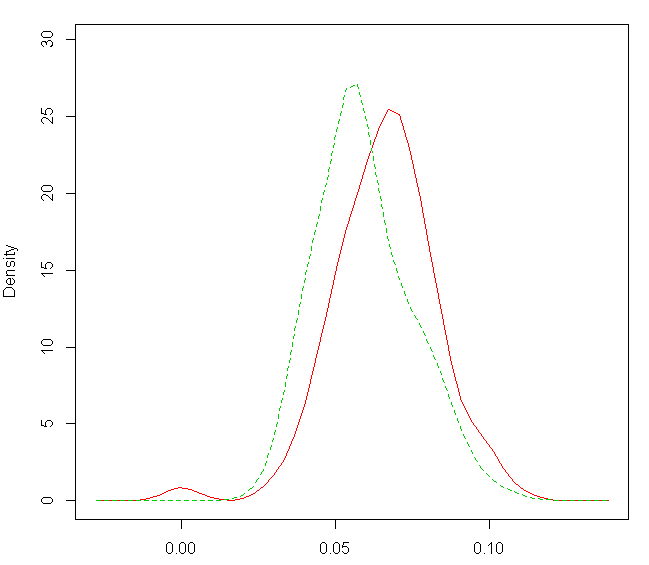
Density plots. Green is reference sample

Distributions seem normal but a normality test says otherwise:

shapiro.test(X[[44]][,8])

        Shapiro-Wilk normality test

data:  X[[44]][, 8] 
W = 0.9693, p-value = 1.748e-06

shapiro.test(X[[45]][, 8])

       Shapiro-Wilk normality test

data:  X[[45]][, 8] 
W = 0.9782, p-value = 0.002443

From the density plot, visually I would say that the two distributions are not different, since they are both within my limits (between 0 and 0.17) and nearly overlapping. In fact the red distribution seems to follow pretty well the reference distribution, which is what I expected.

But if I test this formally, I get that there is a significant shift in the distributions.

t.test(X[[44]][,8],X[[45]][,8]) #regardless of non-normality since sample size is rather large

        Welch Two Sample t-test

data:  X[[44]][, 8] and X[[45]][,8] 
t = 4.7662, df = 470.761, p-value = 2.506e-06
alternative hypothesis: true difference in means is not equal to 0 
95 percent confidence interval:
 0.003906504 0.009387357 
sample estimates:
 mean of x  mean of y 
0.06604217 0.05939524

wilcox.test(X[[44]][,8],X[[45]][,8])

        Wilcoxon rank sum test with continuity correction

data:  X[[44]][, 8] and X[[45]][,8] 
W = 44455.5, p-value = 6.545e-08
alternative hypothesis: true location shift is not equal to 0

ks.test(X[[44]][,8],X[[45]][,8])

        Two-sample Kolmogorov-Smirnov test

data:  X[[44]][, 8] and X[[45]][,8] 
D = 0.2584, p-value = 6.951e-08
alternative hypothesis: two-sided

I also used the method proposed by Harrell-Davis in case comparing quantiles would show that in fact they are similar, but also got statistical differences (see http://www.r-bloggers.com/comparing-all-quantiles-of-two-distributions-simultaneously/).

qcomhd(X[[44]][,8],X[[45]][,8], q = seq(.1, .9, by=.1))
q  n1  n2      est.1      est.2 est.1_minus_est.2        ci.low      ci.up      p_crit p.value signif
1 0.1 332 210 0.04670665 0.04048838       0.006218272  0.0026910365 0.00928384 0.016666667   0.001    YES
2 0.2 332 210 0.05333198 0.04579936       0.007532620  0.0036450303 0.01091243 0.012500000   0.000    YES
3 0.3 332 210 0.05827195 0.05148210       0.006789846  0.0038079921 0.01072252 0.010000000   0.000    YES
4 0.4 332 210 0.06297303 0.05443425       0.008538777  0.0057801177 0.01134807 0.008333333   0.000    YES
5 0.5 332 210 0.06700634 0.05719850       0.009807839  0.0071635533 0.01236572 0.007142857   0.000    YES
6 0.6 332 210 0.07026849 0.06059111       0.009677378  0.0062359534 0.01242078 0.006250000   0.000    YES
7 0.7 332 210 0.07382629 0.06592428       0.007902005  0.0037463285 0.01219320 0.005555556   0.000    YES
8 0.8 332 210 0.07889714 0.07283984       0.006057305  0.0013907057 0.01080278 0.025000000   0.009    YES
9 0.9 332 210 0.08528227 0.08124071       0.004041560 -0.0004749558 0.00909416 0.050000000   0.079     NO

It seems that I am kind of looking for a method that would say what I want to say, but maybe I am biasing my analysis. Is there a reasonable justification (maybe statistically sound) that I can say to back my idea of both samples being comparable?

Thanks for any input