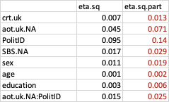
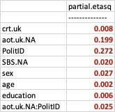
TLDR: This question is about the difference among six R functions with a similar name. The trick to finding the answer is to read their documentation. However, six functions is a bit much; and it's better anyway to know one function but to know it well, so I focus on DescTools::EtaSq. The process (reading the documentation to learn what a function does) is straightforward to apply to the other functions.
Let's start with the definition of eta-squared $\eta^2$ and partial eta-squared $\eta^2_p$. These quantities are measures of effect size and they extend the squared correlation $r^2$ to models with more than one predictor.
$$
\begin{aligned}
\eta^2 &=
\frac{\operatorname{SS}_{\text{effect}}}{\operatorname{SS}_{\text{total}}} =
\frac{\operatorname{SS}_{\text{effect}}}{\sum_i\left(y_i-\bar{y}\right)^2} \\
\eta^2_p &=
\frac{\operatorname{SS}_{\text{effect}}}{\operatorname{SS}_{\text{effect}} + \operatorname{SS}_{\text{error}}} =
\frac{\operatorname{SS}_{\text{effect}}}{\operatorname{SS}_{\text{effect}} + \sum_i\hat{e}_i^2}\\
\end{aligned}
$$
where $\bar{y}$ is the average outcome and the $\hat{e}_i$s are the residuals. So $\eta^2$ is the effect size relative to the total variation in the outcome Y, while $\eta^2_p$ is on the scale of the variability which remains after removing the effect of other terms from the denominator. $\eta^2_p$ is considered easier to compare between studies because the total variability $\operatorname{SS}_{\text{total}}$ depends on the study design.
In a simple linear regression, $r^2 = \eta^2 = \eta^2_p$ where $r$ is the Pearson's correlation between the (single) predictor x and the outcome y.
In a multiple linear regression, we use analysis of variance to compute the sums of squares (SS). And there are (at least) three types of sums of squares. Somewhat unhelpfully, they are called type 1, 2 and 3 (or type I, II and III) and they differ in how they partition the total sum of squares. See How to interpret type I, type II, and type III ANOVA and MANOVA? to learn more; here is a summary.
Using the notation from the linked CV post, let's assume that the model is Y ~ A + B + A:B (two main effects + their interaction).
- Type I is sequential and terms are "added" to the model in order, first the main effects, then the interactions; the type I sum of squares are SS(A), SS(B|A), SS(A:B|A,B)
- Type II adjust the contribution of a predictor for other main effects (but not its interactions, if any): SS(A|B), SS(B|A), SS(A:B|A,B)
- Type III attributes to each term (main effect or interaction) its unique contribution. So the sum of squares due to A excludes the effect of the interaction between A and B: SS(A|B,A:B), SS(B|A,A:B), SS(A:B|A,B).
So this explains the differences between the various eta-squared functions: they have different defaults, so they don't use the same SS type to compute (partial) eta-squared. It's best to be explicit and specify the sum of squares type rather than let the software make a choice for you.
Furthermore, the three SS types are not necessarily different. For example, designs of controlled experiments are often balanced so that the terms A, B an A:B are orthogonal to each other and their contributions don't overlap. (In that case, SS(A|B) = SS(A), etc.; so the conditioning and the order don't matter.) This likely won't be the case in an observational study.
For a recommendation, which calculation is most appropriate for a model with interactions, note that the distinction is in how the contribution of the main effects is computed. Type I doesn't seem very convincing as why would the effect size of A depend on whether we fit the model Y ~ A * B or the model Y ~ B * A. So it's probably best to choose either type II or type III. Alternatively (though this doesn't correspond to an "accepted" SS type) pool together the main effect and the interaction(s) of a predictor to estimate its sum of squares and thus its effect size: SS(A|B,A:B) + SS(A:B|A,B). This approach is described in the section Learning From a Saturated Model of Regression Modeling Strategies by Prof. Frank Harrell. (Caution: The application in RMS is to estimate the predictive potential of a predictor, not to estimate its effect size.)
For illustration purposes, I show how to reproduce the output of DescTools::EtaSq by implementing functions to extract the sum of squares from an anova table and compute eta-squared and partial eta-squared. The DescTools::EtaSq's default is type II.
# Fit an ANOVA with the main effects and an interaction.
model <- aov(Y ~ A + B + A:B, data = data)

# Type I sum of squares and partial eta-squared
# DescTools::EtaSq(model, type = 1)
compute_eta_squared(
  extract_sum_squares(model, anova(model))
)
#>     eta.squared partial.eta.squared
#> A    0.15752020          0.29543977
#> B    0.43518845          0.53671296
#> A:B  0.03163959          0.07768294

# Type II sum of squares and partial eta-squared
# DescTools::EtaSq(model, type = 2)
compute_eta_squared(
  extract_sum_squares(model, car::Anova(model, type = 2))
)
#>     eta.squared partial.eta.squared
#> A    0.18269789          0.32721054
#> B    0.43518845          0.53671296
#> A:B  0.03163959          0.07768294

# Type III sum of squares and partial eta-squared
# DescTools::EtaSq(model, type = 3)
compute_eta_squared(
  extract_sum_squares(model, car::Anova(model, type = 3))
)
#>     eta.squared partial.eta.squared
#> A    0.18718333          0.33257224
#> B    0.44662269          0.54315526
#> A:B  0.03163959          0.07768294
The full R code listing:
library("tidyverse")

extract_sum_squares <- function(model, anova) {
  y <- fitted(model) + residuals(model)
  SS <- anova["Sum Sq"]

  SSeffect <- subset(SS, !(rownames(SS) %in% c("(Intercept)", "Residuals")))
  SSerror <- SS["Residuals", ]
  SStotal <- sum((y - mean(y))^2)

  list(
    SSeffect = SSeffect,
    SSerror = SSerror,
    SStotal = SStotal
  )
}

compute_eta_squared <- function(SS) {
  cbind(
    setNames(SS$SSeffect / SS$SStotal, "eta.squared"),
    setNames(SS$SSeffect / (SS$SSeffect + SS$SSerror), "partial.eta.squared")
  )
}

set.seed(1234)

data <-
  crossing(
    ID = seq(8),
    A = factor(1:3),
    B = factor(1:3)
  ) %>%
  mutate(
    Y = as.numeric(A) + as.numeric(B) + rnorm(n())
  )

# "Break" the balanced design by sampling 80% of the rows
# Comment this line out to see that the three SS types are the same when the design is balanced
data <- sample_frac(data, .8)

# For type 3 sum of squares, it is recommended to fit models with
# "sum" factor encoding and centered covariates.
data$A <- C(data$A, "contr.sum")
data$B <- C(data$B, "contr.sum")

# Fit an ANOVA with the main effects and an interaction.
model <- aov(Y ~ A + B + A:B, data = data)

# Type I sum of squares and partial eta-squared
DescTools::EtaSq(model, type = 1)
compute_eta_squared(
  extract_sum_squares(model, anova(model))
)

# Type II sum of squares and partial eta-squared
DescTools::EtaSq(model, type = 2)
compute_eta_squared(
  extract_sum_squares(model, car::Anova(model, type = 2))
)

# Type III sum of squares and partial eta-squared
DescTools::EtaSq(model, type = 3)
compute_eta_squared(
  extract_sum_squares(model, car::Anova(model, type = 3))
)


