I am running Monte-Carlo simulations on a simple DGP of a mixed logit random coefficient model to check if the mlogit and logitr packages are able to recover the true parameters which are determined by the DGP. The DGP is set as follows
$$u_{ntj} = \beta_{x1} * x1_{njt} + \beta_{x2_{n}} * x2_{njt} + \epsilon_{njt}$$
where $u_{ijt}$ describes the latent utility of individual $n$ at time $t$ of alternative $j$, $x1_{njt}$ is an explanatory variable with fixed coefficient, $x2_{njt}$ is an explanatory variable with random coefficient / slope and $\epsilon_{njt} \sim Gumbel(0, {\pi}^2/6)$ is the error term. $\beta_{x1}$ is the fixed coefficient belonging to $x1_{njt}$ and $\beta_{x2_{n}}$ is the random coefficient belonging to $x2$.
For ease of simplicity, I set $(x1,x2) \sim \mathbf{N}(\mathbf{0}, \mathbf{\Sigma})$ where $\mathbf{\Sigma} = \mathbf{I_2}$ , $\beta_{x2_{n}} \sim \mathbf{N}(\mu_{x2}, \sigma_{x2})$ and $\beta_{x1} = \mu_{x2} = \sigma_{x2} = 1$.
I set the number of Monte-Carlo repetitions / iterations $I = 100$ and varied the number of individuals $N$ between $1000, 5000, 10000$.
The R code I used is as follows:
# Load necessary packages
library(dplyr)
library(mlogit)
library(logitr)
library(EnvStats)
library(parallel)

# Define functions
estimate_mixed_logit <- function(seed, N, T, J, beta_x1, mean_x2, sd_x2, nummultistarts){

  # Setting parameters
  set.seed(seed)

  id <- seq(1:N)
  t <- seq(1:T)
  alt <- seq(1:J)

  # Creation of the data frame
  df <- expand.grid(id, t, alt)
  names(df) <- c('id', 't', 'alt')

  df <- df %>%
    group_by(id) %>%
    mutate(ran_coef = rnorm(1,mean_x2,sd_x2)) %>%
    group_by(id,t,alt) %>%
    mutate(x1 = rnorm(1),
           x2 = rnorm(1),
           e = rgevd(1),
           y_star = case_when(alt == 1 ~ 0 + beta_x1 * x1 + ran_coef * x2 + e,
                              alt == 2 ~ 0 + beta_x1 * x1 + ran_coef * x2 + e,
                              alt == 3 ~ 0 + beta_x1 * x1 + ran_coef * x2 + e)
    ) %>%
    group_by(id,t) %>%
    mutate(max_y_star = max(y_star),
           choice = ifelse(max_y_star == y_star,1,0),
           id_t = cur_group_id()) %>%
    arrange(id,t,alt) %>%
    ungroup()

  # Mlogit estimation

  ## Reshaping the data in mlogit format
  df_cm <- dfidx(df,
                 idx = list(c('id_t','id')),
                 chid.var = 'id',
                 alt.var = 'alt',
                 group.var = 't',
                 choice = 'choice',
                 drop.index = TRUE)

  ## Estimation
  rpar <- c('n')
  names(rpar) <- c('x2')

  mlm <- mlogit(choice ~ 1 + x1 + x2, data = df_cm, panel = TRUE, correlation = FALSE, rpar = rpar)

  # Logitr estimation
  logitr <- logitr(
    data     = df,
    outcome  = 'choice',
    obsID    = 'id_t',
    panelID  = 'id',
    pars     = c('x1', 'x2'),
    randPars = c(x2 = 'n'),
    numMultiStarts = nummultistarts
  )

  return(c(mlm$coefficients[['x1']], mlm$coefficients[['x2']], mlm$coefficients[['sd.x2']],
       logitr$coefficients[['x1']], logitr$coefficients[['x2']], logitr$coefficients[['sd_x2']], logitr$status))


}


# Set global parameters
R <- 100

N <- 1000
T <- 20
J <- 3

beta_x1 <- 1
mean_x2 <- 1
sd_x2 <- 1

nummultistarts <- 30


# Run Monte Carlo simulations
res <- mclapply(1:R,
                mc.cores = 39,
                N = N,
                T = T,
                J = J,
                beta_x1 = beta_x1,
                mean_x2 = mean_x2,
                sd_x2 = sd_x2,
                nummultistarts = nummultistarts,
                FUN <- function(r, N, T, J, beta_x1, mean_x2, sd_x2, nummultistarts){
                  return(estimate_mixed_logit(seed = r,
                                              N = N,
                                              T = T,
                                              J = J,
                                              beta_x1 = beta_x1,
                                              mean_x2 = mean_x2,
                                              sd_x2 = sd_x2,
                                              nummultistarts = nummultistarts
                                              ))
                }
)

# Summarize the results
res <- as.data.frame(do.call(rbind, res))
names(res) <- c('mlogit_beta_x1', 'mlogit_mean_x2', 'mlogit_sd_x2',
                'logitr_beta_x1', 'logitr_mean_x2', 'logitr_sd_x2', 'logitr_status')
which returns the following results:
- N = 1000
summary(res1000)
 mlogit_beta_x1   mlogit_mean_x2    mlogit_sd_x2    logitr_beta_x1   logitr_mean_x2    logitr_sd_x2    logitr_status
 Min.   :0.9701   Min.   :0.8299   Min.   :0.9425   Min.   :0.9720   Min.   :0.9312   Min.   :-1.154   Min.   :3
 1st Qu.:0.9886   1st Qu.:0.9569   1st Qu.:1.0069   1st Qu.:0.9902   1st Qu.:1.0215   1st Qu.: 1.042   1st Qu.:3
 Median :0.9986   Median :0.9757   Median :1.0370   Median :1.0005   Median :1.0499   Median : 1.065   Median :3
 Mean   :0.9984   Mean   :0.9724   Mean   :1.0352   Mean   :1.0004   Mean   :1.0476   Mean   : 1.021   Mean   :3
 3rd Qu.:1.0085   3rd Qu.:0.9903   3rd Qu.:1.0568   3rd Qu.:1.0096   3rd Qu.:1.0738   3rd Qu.: 1.090   3rd Qu.:3
 Max.   :1.0326   Max.   :1.0692   Max.   :1.1166   Max.   :1.0335   Max.   :1.1218   Max.   : 1.155   Max.   :3
- N = 5000
summary(res5000)
 mlogit_beta_x1   mlogit_mean_x2    mlogit_sd_x2    logitr_beta_x1   logitr_mean_x2    logitr_sd_x2    logitr_status
 Min.   :0.9784   Min.   :0.9314   Min.   :0.9788   Min.   :0.9805   Min.   :0.9504   Min.   :-1.115   Min.   :3
 1st Qu.:0.9929   1st Qu.:0.9592   1st Qu.:1.0191   1st Qu.:0.9949   1st Qu.:1.0424   1st Qu.: 1.052   1st Qu.:3
 Median :0.9986   Median :0.9720   Median :1.0308   Median :1.0003   Median :1.0534   Median : 1.059   Median :3
 Mean   :0.9979   Mean   :0.9715   Mean   :1.0315   Mean   :0.9998   Mean   :1.0525   Mean   : 1.038   Mean   :3
 3rd Qu.:1.0025   3rd Qu.:0.9836   3rd Qu.:1.0434   3rd Qu.:1.0042   3rd Qu.:1.0614   3rd Qu.: 1.071   3rd Qu.:3
 Max.   :1.0119   Max.   :1.0197   Max.   :1.0691   Max.   :1.0135   Max.   :1.1003   Max.   : 1.092   Max.   :3
- N = 10000
summary(res10000)
 mlogit_beta_x1   mlogit_mean_x2    mlogit_sd_x2   logitr_beta_x1   logitr_mean_x2   logitr_sd_x2   logitr_status
 Min.   :0.9839   Min.   :0.9412   Min.   :1.002   Min.   :0.9858   Min.   :1.027   Min.   :1.031   Min.   :3
 1st Qu.:0.9930   1st Qu.:0.9596   1st Qu.:1.021   1st Qu.:0.9952   1st Qu.:1.044   1st Qu.:1.051   1st Qu.:3
 Median :0.9960   Median :0.9664   Median :1.028   Median :0.9978   Median :1.051   Median :1.060   Median :3
 Mean   :0.9962   Mean   :0.9666   Mean   :1.029   Mean   :0.9981   Mean   :1.050   Mean   :1.059   Mean   :3
 3rd Qu.:0.9997   3rd Qu.:0.9732   3rd Qu.:1.037   3rd Qu.:1.0018   3rd Qu.:1.056   3rd Qu.:1.067   3rd Qu.:3
 Max.   :1.0050   Max.   :0.9916   Max.   :1.055   Max.   :1.0069   Max.   :1.082   Max.   :1.082   Max.   :3
whereby I ensured that all maximum likelihood estimations achieved convergence, see logitr_status for instance.
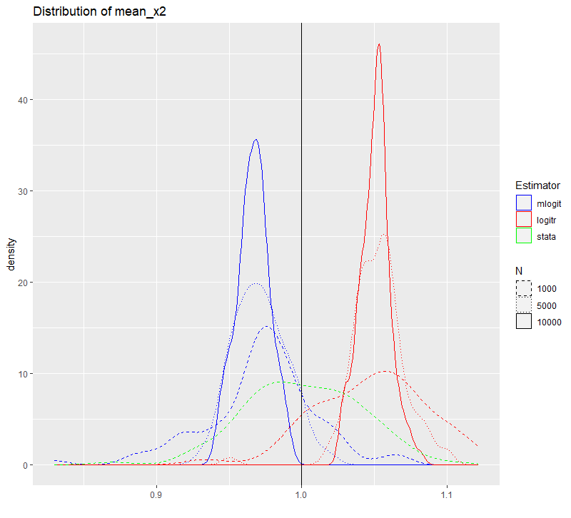
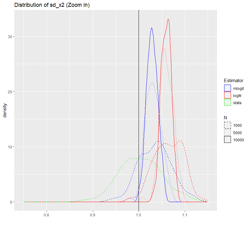
My results suggest that both mlogit and logitr estimates for $x2$ are biased and even inconsistent since they do not converge to the true parameters for $x2$, i.e. $\mu_{x2}$ and $\sigma_{x2}$ when increasing $N$. When running the Monte-Carlo simulation in Stata using the exact same data ($N = 1000$) and the command cmmixlogit choice x1, random(x2), I obtain unbiased results, see the following:
summary(stata1000)
 stata_beta_x1    stata_mean_x2     stata_sd_x2     stata_converged
 Min.   :0.9716   Min.   :0.8698   Min.   :0.8857   Min.   :1
 1st Qu.:0.9918   1st Qu.:0.9731   1st Qu.:0.9728   1st Qu.:1
 Median :0.9997   Median :0.9990   Median :1.0033   Median :1
 Mean   :1.0015   Mean   :1.0007   Mean   :1.0063   Mean   :1
 3rd Qu.:1.0107   3rd Qu.:1.0292   3rd Qu.:1.0345   3rd Qu.:1
 Max.   :1.0407   Max.   :1.1016   Max.   :1.1531   Max.   :1
Does anybody have an explanation for this outcome or is there a conceptual misunderstanding in my set-up? My best guess is that Stata’s numeric optimization outperforms the ones of both R packages. However, I am surprised that this seems to lead to biased + inconsistent estimates (in finite samples up to $N = 10000$).
P.S.: I am aware of this post (mlogit package fails to recover synthetic mixed logit model) but changing the optimization method / algorithm to the BHHH algorithm (for the mlogit package) or the number of draws mlogit R argument set to 100) didn’t affect the outcome of bias and inconsistency in my case.
Update August 24th 2023:
Thanks @jhelvy for your reply and support!
According to https://cran.r-project.org/web/packages/mlogit/mlogit.pdf mlogit's default value of draws is 40.
Stata’s cmmixlogit is by default using the Hammersley instead of the Halton sequence for the generation of point sets used in the Monte Carlo integration. Moreover, it uses a flexible number of integration points / draws: $500 + \lfloor 2.5 \sqrt{N_c (\ln(r + 5) + v)}\rfloor$, where $N_c$ is the number of cases, $r$ is the number of random coefficients in the model, and $v$ is the number of variance parameters, see https://www.stata.com/manuals/cmcmmixlogit.pdf.
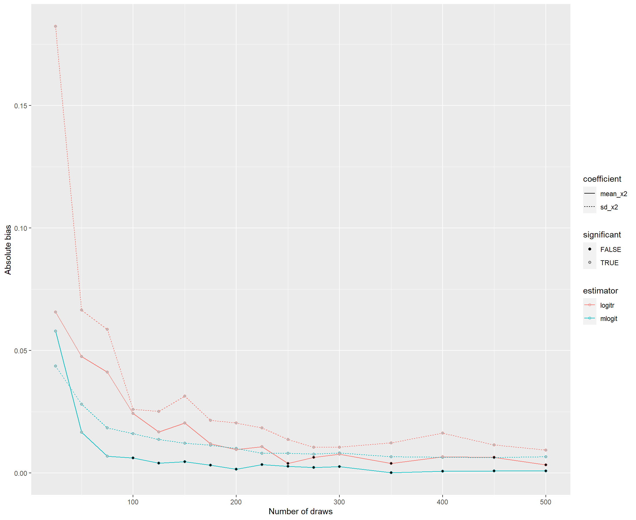
As you have suggested I replicated my analysis ($N = 1000$, $R = 100$, same DGP as described above) for varying number of draws. The following chart shows the mean absolute deviation across the $R$ number of iterations to the true parameter value for different levels of draws. The significance test refers to an one sample t test testing the null hypothesis that the respective mean of the absolute bias is statistically significant from zero with $\alpha =0.05$. TRUE / FALSE are representing that the respective p-value of this test below / above 10%.

My conclusion from this additional analysis is that 200 draws seems to be an adequate number to offset the tradeoff between bias and computation time. However, I am wondering that even for 500 draws there is still some statistically significant bias and that logitr seems to be performing less than mlogit. @jhelvy Do you have an explanation for this?
My understanding is that mlogit uses pseudo-random numbers in contrast to Halton sequences. Is this maybe explaining the difference although I would expect it to be the opposite, see Chapter 9 of the textbook by Kenneth Train.
Finally, you’re absolutely right regarding the necessity to take the absolute value for the sd_x2 parameter. I changed it in my code and ensured that this does not affect my previous results.
Update August 28th 2023:
I run some additional Monte-Carlo simulations where I (i) altered the distribution of x2 from normal to log-normal and (ii) switched from preference to willingness-to-pay (WTP) space estimation mererly using the logitr package. For the latter, I altered the DGP by introducing a new variable $x3 \sim \mathbf{N}(0, 1)$ with $\beta_{x3_{n}} = -1$ which can be viewed as the price which enters negatively into the utility function: $$u_{ntj} = \beta_{x1} * x1_{njt} + \beta_{x2_{n}} * x2_{njt} + \beta_{x3_{n}} * x3_{njt} + \epsilon_{njt}$$
Rewriting to the WTP space expression gives: $$u_{ntj} = \lambda_n ( \omega_{x1} * x1_{njt} + \omega_{x2_{n}} * x2_{njt} - x3_{njt}) + \epsilon_{njt}$$ where $\lambda_n = \beta_{x3_{n}}$ de facto since I set $\sigma_{\epsilon} = 1$, see above.
The following table shows the results by specification where for all simulations $N = 1000$ and $R = 100$ and only the estimates of converged iterations $r$ have been taken into account.
| Space | Distribution $\beta_{x2}$ | Distribution $\lambda$ | Number of Draws | Number of logitr multistarts |
mlogit bias $\beta_{x1}$ |
mlogit bias $\mu_{\beta_{x2}}$ |
mlogit bias $\sigma_{\beta_{x2}}$ |
mlogit convergence rate |
logitr bias $\beta_{x1}$ |
logitr bias $\mu_{\beta_{x2}}$ |
logitr bias $\sigma_{\beta_{x2}}$ |
logitr bias $\lambda$ / $\mu_{\lambda}$ |
logitr bias $\sigma_{\lambda}$ |
logitr convergence rate |
|---|---|---|---|---|---|---|---|---|---|---|---|---|---|---|
| Preference | $\mathbf{Lognormal}(1,1)$ | 200 | 30 | 0% | 5% | 1% | 100% | 0% | 1% | 1% | 52% | |||
| Preference | $\mathbf{Lognormal}(1,1)$ | 500 | 200 | 0% | 8% | 0% | 100% | 0% | 0% | 0% | 64% | |||
| WTP | $\mathbf{N}(1,1)$ | fixed to $\lambda$ = 1 | 200 | 30 | 0% | 4% | 1% | 0% | 100% | |||||
| WTP | $\mathbf{N}(1,1)$ | $\mathbf{N}(1,1)$ | 200 | 30 | 0% | -7% | 6% | -5% | 819% | 100% | ||||
| WTP | $\mathbf{N}(1,1)$ | $\mathbf{Lognormal}(1,1)$ | 200 | 30 | 0% | -4% | 4% | -2% | 2% | 100% | ||||
| WTP | $\mathbf{Lognormal}(1,1)$ | fixed to $\lambda$ = 1 | 200 | 30 | 0% | -2% | 1% | 0% | 95% | |||||
| WTP | $\mathbf{Lognormal}(1,1)$ | $\mathbf{N}(1,1)$ | 200 | 30 | 0% | 2% | 1% | -9% | 831% | 68% | ||||
| WTP | $\mathbf{Lognormal}(1,1)$ | $\mathbf{Lognormal}(1,1)$ | 500 | 200 | 0% | -2% | 1% | -1% | 6% | 22% |
From my point of view, there are three key findings:
mlogitestimates for $\mu_{\beta_{x2}}$ in the preference space when $x2 \sim \mathbf{Lognormal}(1,1)$ seem to considerably deviate.logitrestimates for $\mu_{\beta_{x2}}$ and $\sigma_{\beta_{x2}}$ in the WTP space when $x2 \sim \mathbf{N}(1,1)$ seem to considerably deviate independent from the distribution of $\lambda$.logitrestimates for the nuisance parameter of $\lambda$ can be heavily biased which are, however, of less interest.
Any thoughts on these additional insights?


mlogitwith pseudo random numbers draws (the default) tomlogitwith halton draws and (ii)logitrwith halton draws tologitrwith sobol draws. For number of draws equal to 200 there is no real difference detectable in the estimates among the two groups. For number of draws equal to 100, there is again no difference for themlogitestimators but the sobol draw variant oflogitrperforms slight less than the halton variant. $\endgroup$cmmixlogitperforms if I force it to just use 100 draws of either the Hammersley sequence (the default) or the Halton sequence. Both are unbiased thanmlogitorlogitrvariants even for this number of draws. $\endgroup$