The number of places in which two 0-1 arrays A and B (of the same length) both have ones is readily computed as
=SUMPRODUCT(A,B)
This generalizes: for three 0-1 arrays A, B, and C use =SUMPRODUCT(A,B,C), and so on.
The rest is a matter of systematically referencing all possible combinations of your variables so that you don't have to write $2^5=32$ different such formulas. To this end, I will suppose the data are organized in a standard way: each variable is a column; the first row in each column contains the variable name; no rows are blank or skipped; and all columns have the same number of entries. I will further suppose these data are contiguous so that they form a rectangular array.
In Excel, as in almost all computing systems, it is advantageous to use meaningful names for data. Let us, then, name this array of data (without its first row of names) Data. We will want to be able to index the columns by numbers. Excel prefers to start indexes with $0$, so that the zeroth index will be the leftmost column, index $1$ will refer to the second-to-the-left, and so on. Although there are various ways to do this, a convenient one uses OFFSET: OFFSET(Data, 0, 0, , 1) is the left column of data, OFFSET(Data, 0, 1, , 1) is the next column, and so on. You can see that the third argument of OFFSET is the one that picks out the column. In this way, for instance, the formula
=SUMPRODUCT(OFFSET(Data,0,0,,1), OFFSET(Data,0,1,,1))
computes the number of places in which the leftmost two columns (with indexes $0$ and $1$) both have ones.
The formulas still vary too much: they will have between two and five arguments, depending on how many columns are involved. To make things easier to enter, I suggest a little trick: create a column of all ones. It must have exactly the same number of entries as all the others, but it need not be contiguous with them: let's simply name it One. When you treat this as if it were are variable, including it in the SUMPRODUCT formula changes nothing. Therefore, we can write a single formula involving all five columns in which each column is used when needed and otherwise is replaced by the column of ones. Here is the formula (created with a lot of copy-and-paste, of course, so it's not as difficult to write as it might look):
=SUMPRODUCT(IF(MID(I2,1,1)="1", OFFSET(Data,0,0,,1), One),
            IF(MID(I2,2,1)="1", OFFSET(Data,0,1,,1), One),
            IF(MID(I2,3,1)="1", OFFSET(Data,0,2,,1), One),
            IF(MID(I2,4,1)="1", OFFSET(Data,0,3,,1), One),
            IF(MID(I2,5,1)="1", OFFSET(Data,0,4,,1), One))
The expressions MID(I2,1,1), etc, are binary codes "00000", "00001", "00010", ..., through "11111" indicating all possible combinations of the columns "A" through "E". They are easy to generate from a list of the integers $0, 1, \ldots, 2^5-1=31$ using the DEC2BIN function. MID picks out each binary digit in turn. The IF expressions use the corresponding column for the calculation whenever the digit is a $1$ and otherwise use the default column of ones, as explained.
To make this more readable we may also choose to convert the binary codes into lists of their corresponding columns. Because that's a peripheral detail, I won't go into the method here, but you can see it in the screenshots below.
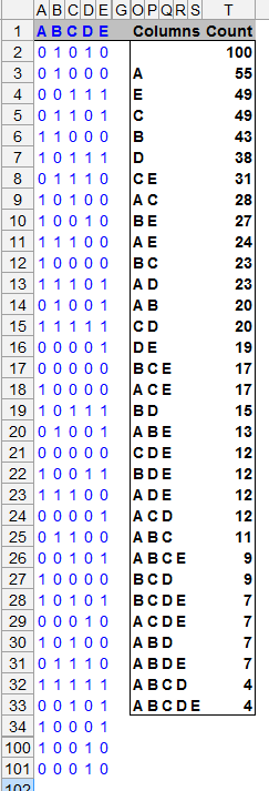
Upon hiding some of the intermediate calculations and sorting the results (COUNT) in descending order, the spreadsheet will look like this:

The first value of Count tells us how many data rows there are. The entries for "A", "B", ..., "E" count the total numbers of ones for each variable. After them come the entries for combinations of variables. E.g., "C" and "E" have $31$ ones in common, then "A" and "C" have $28$ in common, and so on. I believe this is the information the question asks for. It is one way to represent a $2^5$ cross-tabulation.
The blue text, by the way, indicates original (raw) data. The bold black text displays the results. Intermediate calculations, shown below, are neither blue nor bold.

Index was a list of $0, 1, \ldots, 2^5-1$ before the results were sorted by decreasing Count. Code is its base-2 representation. The next five columns (J:N) are used ultimately to show the information under the Columns header: which variables are designated by each Code.
All formulas are the same in each row: they were entered in the first data row and then just propagated down through 31 more rows to complete the table before it was sorted. Moreover, the formulas appear in two groups of five: columns J:N and columns O:S. Those were created from a single formula each, copied, pasted, and suitably modified for each column. Here they are:

Those wishing to compare this solution with those developed using a statistical computing platform, consider this one in R, whose input x is a data frame object with (at least) five columns:
b <- c(FALSE,TRUE)
subsets <- as.matrix(expand.grid(A=b, B=b, C=b, D=b, E=b))
rownames(subsets) <- apply(subsets, 1, function(i)
    paste(colnames(x)[i, drop=FALSE], sep="", collapse=""))
sort(apply(subsets, 1, function(i)
    sum(apply(x[, i, drop=FALSE], 1, function(y) min(c(1,y)) > 0))), decreasing=TRUE)
You can see the same computations happening (although some of the details are buried in expand.grid, just as I buried them in the hidden columns of the spreadsheet, and the product of ones and zeros has been replaced by a check of their minimum value because that's simpler to code in R). I find the Excel solution convenient to implement when the data are already in a spreadsheet, but it is a little risky to code and rather difficult and unreliable to apply to another dataset whose dimensions might be different or which might have missing values.


