Is there a way to calculate LC50 from a continuous dependent variable?

Question

I'm very new to R and also statistics, so the basics are lost on me. In the past I have done some simple experiments with chemicals and calculating the LC50 from binary responses (dead or alive). However, this time, I must calculate the LC50 from continuous response variables; for example: toxicant concentrations (independent variable) by absorbance values of a metabolic compound (continuous dependent variable). How do I go about doing this? I need to obtain the LC50 to be able to perform sublethal tests with the toxicants.

I've read around I'm not sure if it's a good idea to normalise these values as a percentage of the untreated control group then do a regression because of potential information loss(?)

I'll appreciate any suggestions and insight.

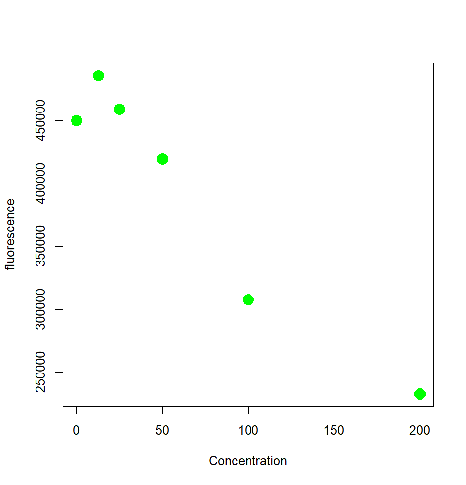
EDIT1: Thanks for the responses. Honestly I am even more confused now as I don't understand how to perform these tasks or what I am doing wrong when I attempt it in R. I've tried @Ben Bolker's suggestion and got a negative xmid. Forgive me if the format is not correct but here is a direct copy of the code I used and bit more information about the data: I have 6 test concentrations from 0 up to 200 mg/L and 18 observations per treatment (n=3).

I entered the following lines of code:

plot(PU$Concentration, PU$fluorescence, xlab="Concentration", ylab="fluorescence",col="green", pch=19, cex=2)

testmodel<-nls(fluorescence~SSlogis(Concentration,Asym,xmid,scal), data=PU) summary(testmodel)

This was the output:

_Formula: fluorescence ~ SSlogis(Concentration, Asym, xmid, scal)

Parameters: Estimate Std. Error t value Pr(>|t|) Asym 1319849.9 2757240.6 0.479 0.633 xmid -106.6 711.0 -0.150 0.881 scal -192.9 151.6 -1.272 0.206

Residual standard error: 98540 on 105 degrees of freedom

Number of iterations to convergence: 0 Achieved convergence tolerance: 4.008e-06_

How would one interpret this? How can the xmid be negative?

Answer 1

What you describe is a concentration-response curve, curves that in my experience more typically involve continuous rather than binary (alive/dead) outcomes. With a continuous response/outcome the value you seek is typically called "IC50" (concentration for 50% inhibition) or "EC50" (concentration for 50% effect) rather than the "LC50" (concentration for 50% lethality) that better describes alive/dead outcomes.

A typical best practice is to fit all the data, in your case absorbance versus toxicant concentration, with a nonlinear least squares regression model that captures the underlying dynamics. Then estimate the concentration at which the absorbance is half way between the model's estimates of the lower and upper asymptotes. If your lower asymptote is necessarily 0 and a simple logistic model is appropriate, then Ben Bolker's suggestion of a simple 3-parameter nls() model with a SSlogis() equation form might be OK.

If this is something like the MTT assay, however, there's a chance that there will be positive absorbance even when all the cells have died. Then you need to model both the upper and lower asymptotes. Also, depending on the way the toxicant affects cell metabolism or death, a simple logistic model might not capture the curve between the asymptotes if there is an asymmetry around the midpoint.

There is a drc package in R that handles many forms of dose-response curves. For example, it can fit a 5-parameter logistic model that models both the asymptotes and the asymmetry, or a model that handles hormesis, a biphasic concentration-response curve that can occur in practice when small doses of a "toxicant" might actually increase metabolism. Using this package takes some care, however, as fitting a nonlinear regression only works reliably if you have good starting estimates for the model parameters.

A common beginner's mistake is just to submit the data to the software without looking at the concentration-response curve carefully, first. Always plot the data. Always look at how well the model fits.

There are additional biological considerations you should know about: the IC50 in an MTT-type assay doesn't always measure what you think it does. A review in Int. J. Mol. Sci. 2021, 22(23), 12827 discusses those matters, off-topic on this site.