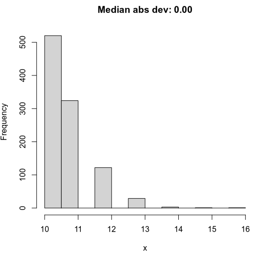
Heavily borrowing from previous answers, here's an example:
set.seed(1)
x <- 10 + rpois(1000, lambda=log(2))
Histogram of variable x
xmad <- mad(x)
hist(x, main=sprintf('Median abs dev: %.2f', xmad))

If you count the distinct values in x you see that 10 makes up more than 50% of the datapoints:
# Counts of distinct values in x
table(x)
x
 10  11  12  13  14  15  16
520 324 122  29   3   1   1

# As percentage
table(x) / length(x)
x
   10    11    12    13    14    15    16
0.520 0.324 0.122 0.029 0.003 0.001 0.001
This means that more than 50% of the values will have absolute deviation of 0 and therefore the median absolute deviation from the median of x will be 0.
Here's another random draw from the same distribution where instead the mad is different from zero:
set.seed(1234)
x <- 10 + rpois(1000, lambda=log(2))
mad(x)
[1] 1.48

table(x)
x
 10  11  12  13  14  15
482 358 117  37   5   1

table(x) / length(x)
x
   10    11    12    13    14    15
0.482 0.358 0.117 0.037 0.005 0.001

