3
$\begingroup$

I'm struggling to develop a deep intuition for why monotonic transformations preserve relative probabilities in continuous cases. While I understand the idea at a surface level, particularly for discrete cases (where it's easier to think in terms of counts), I lose my intuition when trying to extend this to continuous distributions.

I think I understand the following so far:

  1. A monotonic transformation $f(x)$ (e.g., $f(x) = x^2$ on $x \geq 0$) preserves the order of outcomes. If $x_1 < x_2$, then $f(x_1) < f(x_2)$.
  2. In discrete cases, this order preservation combined with the one-to-one nature of the mapping helps me see why relative probabilities don’t change—the counts remain proportional, even though the values are transformed.
  3. In continuous cases, the probability density function (PDF) changes according to the derivative of the transformation: $$p_Y(y) = p_X(f^{-1}(y)) \cdot \left| \frac{d}{dy} f^{-1}(y) \right|,$$ where $f^{-1}(y)$ is the inverse of $f(x)$. But I’m having trouble connecting this formula to an intuitive/visual understanding of why relative probabilities over intervals remain unchanged.

Where I get stuck:

  1. For transformations like $f(x) = x^2$, which stretches the input space non-uniformly (e.g., $1 \to 1, 2 \to 4, 10 \to 100$), it feels like the larger values might disproportionately dominate the probability. For example, the interval $[10, 11]$ maps to $[100, 121]$, which is much larger than $[1, 2] \to [1, 4]$.
  2. My intuition breaks down because I struggle to reconcile how the adjustment by the derivative $\frac{1}{f'(x)}$ (or $\frac{1}{2\sqrt{y}}$ for $f(x) = x^2$) "balances" this stretching effect. In a discrete case i can imagine the one to one mapping as simple a relabelling where relative counts stay the same. But for the continuous case i can't find the same satisfaction.

What I’d like to understand:

  1. How does the change-of-variables formula ensure that relative probabilities (e.g., $P(Y \in [a, b]) / P(Y \in [c, d])$) are preserved under monotonic transformations? Is there a way to build intuition for this beyond just trusting the formula?
  2. How should I think about this transformation geometrically? Does it help to think of probabilities as "density mass" that gets redistributed, and if so, why does this redistribution not distort the relative sizes?
  3. Are there specific examples or visualisations that might help bridge my intuition gap, particularly for continuous distributions?

Thank you for any insights!

Update

As Whuber kindly pointed out my initial assumption/question is wrong which is maybe why it is confusing me. I have attached bellow a reference I was clearly misinterpreting to arrive at this conclusion. Thoughts still very much appreciated.

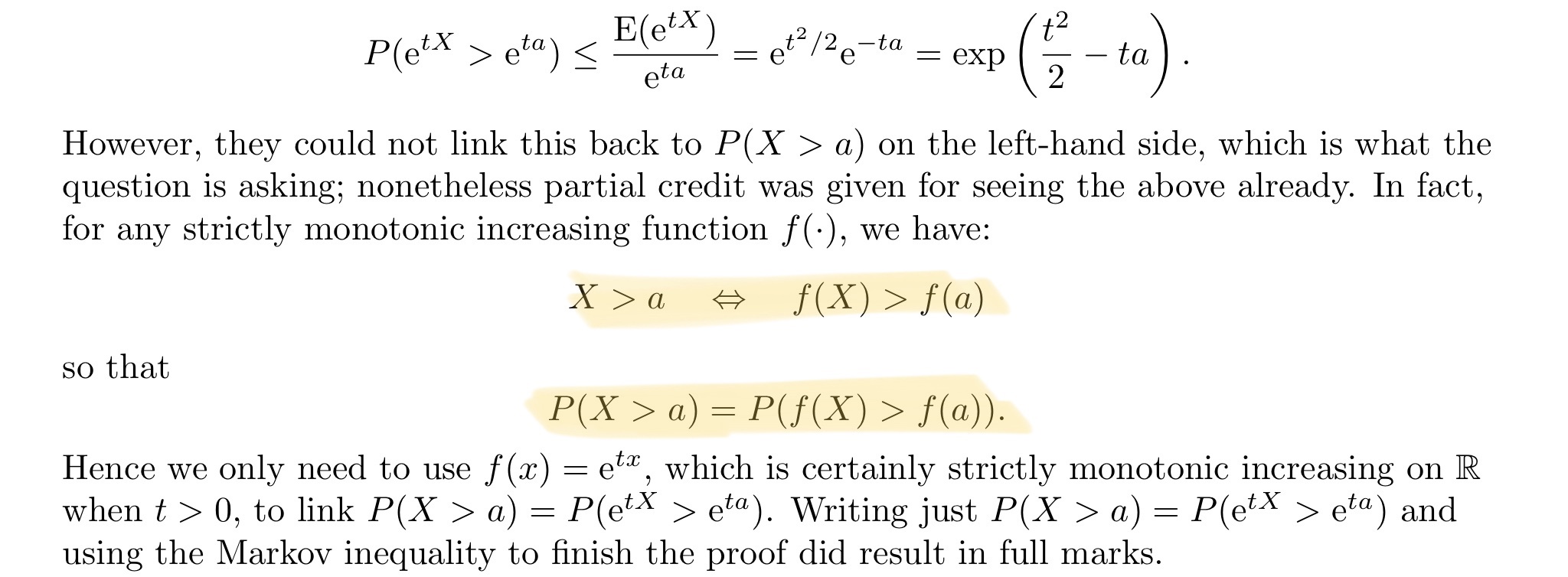
enter image description here

$\endgroup$
8
  • 1
    $\begingroup$ Your question (1) doesn't even employ a transformation, making it difficult to interpret. Maybe you are looking for something like stats.stackexchange.com/questions/14483? Regardless, monotonic transformations generally do not preserve probabilities or even probability densities. $\endgroup$
    – whuber
    Commented Dec 4 at 21:45
  • 1
    $\begingroup$ This question is cross-posted at SE.math (math.stackexchange.com/questions/5007245). $\endgroup$
    – Ben
    Commented Dec 5 at 1:14
  • $\begingroup$ Hi Ben, thank you very much for your answer! Will digest it soon. Apologies, I did cross post this. Sometimes the forums have been very slow so I was trying to maximise my chances, and honestly the range of different answers is really helpful For finding that thing that “clicks.” $\endgroup$
    – CormJack
    Commented Dec 6 at 1:25
  • $\begingroup$ Thanks for your comments as always Whuber. I agree with both points and I have emended the end of the question. I think the example I have provided captures the idea I was trying to get and failing. it seems like there is some relative preservation? Again I’m not sure so your thoughts interpreting the attached, and the difference between this and preserving probabilities would be appreciated. Thanks! $\endgroup$
    – CormJack
    Commented Dec 6 at 1:53
  • $\begingroup$ @whuber are you able to help me understand your comment note in light of the image I’ve attached at the end of the post, and also the other comments which seem to support some notion of monophonic transformations preserving probabilities. Apologies if my terminology is off, I’d greatly appreciate your insight when you get a sec! $\endgroup$
    – CormJack
    Commented Dec 11 at 11:26

2 Answers 2

3
$\begingroup$

Consider the continuous case over a "small" interval

To obtain intuition about continuous random variables and functions, it often helps to consider them over "small" enough intervals where continuous functions and densities are roughly constant. The "small" quantities used for the intervals can then act as differentials when you make them smaller and smaller. (Much of this explanation will rely on the limiting definition of a derivative and the corresponding approximation to a derivative over small intervals.)

Suppose you have a continuous random variable $X \sim f_X$ and you apply a monotonic transformation $T: \mathbb{R} \rightarrow \mathbb{R}$ to get the random variable $Y=T(X)$. (We will assume that $T$ is continuous and differentiable so that the probability transform formula applies.) Because of the monotonicity of the transform, for any point $x \in \mathbb{R}$ and any interval length $\Delta x > 0$ we must have the equivalence:

$$\mathbb{P}(x < X \leqslant x + \Delta x) = \mathbb{P}(T(x) < Y \leqslant T(x + \Delta x)).$$

This is the result you are struggling to see intuitively from the relevant probability transformation formula. To get to the intuition, let's consider what happens when the interval length $\Delta x$ is "small" enough that all relevant continuous functions/densities are approximately constant over the relevant interval. Since $T$ is continuous and differentiable, for small $\Delta x >0$ we have the linear approximation:

$$\begin{align} T(x + \Delta x) &= T(x) + [T(x + \Delta x) - T(x)] \\[12pt] &= T(x) + \frac{T(x + \Delta x) - T(x)}{\Delta x} \cdot \Delta x \\[12pt] &\approx T(x) + T'(x) \cdot \Delta x. \\[6pt] \end{align}$$

Taking $y=T(x)$ and $\Delta y = T'(x) \cdot \Delta x$ we then have:

$$\begin{align} f_X(x) \cdot \Delta x &\approx \mathbb{P}(x < X \leqslant x + \Delta x) \\[18pt] &= \mathbb{P}(T(x) < Y \leqslant T(x + \Delta x)) \\[18pt] &\approx \mathbb{P}(T(x) < Y \leqslant T(x) + T'(x) \cdot \Delta x) \\[18pt] &= \mathbb{P}(y < Y \leqslant y + \Delta y) \\[12pt] &= \frac{\mathbb{P}(y < Y \leqslant y + \Delta y)}{\Delta y} \cdot \Delta y \\[10pt] &\approx f_Y(y) \cdot \Delta y. \\[6pt] \end{align}$$

As you can see, the change from $\Delta x$ to $\Delta y$ in this working occurs because of the linear approximation to $T(x + \Delta x)$ using the derivative of the function $T$, which is precisely the behaviour you are describing when you note the "stretching" behaviour that occurs for the quadratic transformation in your example. The length of the relevant interval changes from $\Delta x$ to $\Delta y$ due to the transformation and so each of the densities must be multiplied by the applicable interval lengths to maintain equivalence in probability.

Now, if we imagine the interval length $\Delta x$ getting smaller and smaller (so that $\Delta y$ also gets smaller and smaller) then these approximations become more and more accurate. If we take limits of the interval lengths down to zero then they become differentials and the approximations now hold exactly. We then obtain the general equivalence:

$$f_X(x) \ dx = f_Y(y) \ dy \quad \quad \quad \quad \quad y=T(x) \quad \quad \quad \quad \quad dy = T'(x) \ dx.$$

This is the general equivalence that holds between the densities of $X$ and $Y$ under a monotonic transformation, which ensures that the probabilities over transformed intervals remains constant. The reason that the derivative term appears in the density transformation formula is because the differentials in the equivalence must be different to maintain the balance.

$\endgroup$
0
$\begingroup$

It' easier to build intuition in your case with CDF $F(x)=P(X\le x)$ rather than with the density $f(x)=F'(x)$. Consider this: it must be that $F(x)=F(x^3)$. Then you have $F(x_1^3)<F(x_2^3)$ when $x_1<x_2$

$\endgroup$

Your Answer

By clicking “Post Your Answer”, you agree to our terms of service and acknowledge you have read our privacy policy.

Not the answer you're looking for? Browse other questions tagged or ask your own question.