The econometrics of a Bayesian approach to event study methodology

Question

Event studies are widespread in economics and finance to determine the effect of an event on a stock price, but they are almost always based on frequentist reasoning. An OLS regression -- over a reference period which is distinct from the event window -- is usually used to determine the parameters required to model the normal return for an asset. One then determines the statistical significance of cumulative abnormal returns ($\text{CAR}$) on asset $i$ following an event during a specified event window from $T_1$ to $T_2$. A hypothesis test is used to determine whether these returns are significant and thus indeed abnormal or not. Thus:

$H_0 : \text{CAR}_i = 0$, where

$\text{CAR}_i = \sum_{t=T_1}^{T_2} \text{AR}_{i,t} = \sum_{t=T_1}^{T_2} \left( r_{i,t} -\mathbb{E}[r_{i,t}] \right)$, and

$\mathbb{E}[r_{i,t}]$ is the return on the asset predicted by the model.

If our number of observations is large enough, we can assume asymptotic normality of the distribution of asset returns, but this may not be verified for a smaller sample size.

It can be argued that because of this, single-firm, single-event studies (as required for example in litigation) should follow a Bayesian approach, because the assumption of infinitely many repetitions is much "further from being verified" than in the case of multiple firms. Yet, the frequentist approach remains common practice.

Given the scarce literature on this subject, my question is how to best approach an event study -- analogous to the methodology outlined above and summarised in MacKinlay, 1997 -- using a Bayesian approach.

Although this question arises within the context of empirical corporate finance, it is really about the econometrics of Bayesian regression and inference, and the differences in reasoning behind frequentist and Bayesian approaches. Specifically:

1. How should I best approach the estimation of the model parameters using a Bayesian approach (assuming a theoretical understanding of Bayesian statistics, but little to no experience in using it for empirical research).

2. How do I test for statistical significance, once cumulative abnormal returns have been computed (using the normal returns from the model)?

3. How can this be implemented in Matlab?

Answer 1

As mentioned in the comments, the model you're looking for is Bayesian linear regression. And since we can use BLR to calculate the posterior predictive distribution $p(r_t|t, \mathcal{D}_\text{ref})$ for any time $t$, we can numerically evaluate the distribution $p(\text{CAR}|\mathcal{D}_\text{event}, \mathcal{D}_\text{ref})$.

The thing is, I don't think a distribution over $\text{CAR}$ is what you really want. The immediate problem is that $p(\text{CAR} = 0|\mathcal{D}_\text{event}, \mathcal{D}_\text{ref})$ has probability zero. The underlying problem is that the "Bayesian version of hypothesis tests" is comparing models via their Bayes factor, but that requires you to define two competing models. And $\text{CAR} = 0, \text{CAR} \neq 0$ are not models (or at least, they're not models without some extremely unnatural number juggling).

From what you've said in the comments, I think what you actually want to answer is

Are $\mathcal{D}_\text{ref}$ and $\mathcal{D}_\text{event}$ better explained by the same model or by different ones?

which has a neat Bayesian answer: define two models

• $M_0$: all the data in $\mathcal{D}_\text{ref}, \mathcal{D}_\text{event}$ is drawn from the same BLR. To calculate the marginal likelihood $p(\mathcal{D}_\text{ref}, \mathcal{D}_\text{event}|M_0)$ of this model, you'd calculate the marginal likelihood of a BLR fit to all the data.

• $M_1$: the data in $\mathcal{D}_\text{ref}$ and $\mathcal{D}_\text{event}$ are drawn from two different BLRs. To calculate the marginal likelihood $p(\mathcal{D}_\text{ref}, \mathcal{D}_\text{event}|M_1)$ of this model, you'd fit BLRs to $\mathcal{D}_\text{ref}$ and $\mathcal{D}_\text{event}$ independently (though using the same hyperparameters!), then take the product of the two BLR marginal likelihoods.

Having done that, you can then calculate the Bayes factor

$$\frac{p(\mathcal{D}_\text{ref}, \mathcal{D}_\text{event}|M_1)}{p(\mathcal{D}_\text{ref}, \mathcal{D}_\text{event}|M_0)}$$

to decide which model is more believable.

Answer 2

You cannot do an event study with a single firm.

Unfortunately you need panel data for any event study. Event studies focus on returns for individual time periods before and after events. Without multiple firm observations per time period before and after the event, it's impossible to distinguish noise (firm specific variation) from the effects of the event. Even with only a few firms, noise will dominate event, as StasK points out.

That being said, with a panel of many firms you can still do Bayesian work.

How to estimate normal and abnormal returns

I'm going to assume that the model you use for normal returns looks something like a standard arbitrage model. If it doesn't you should be able to adapt the rest of this discussion. You'll want to augment your "normal" return regression with a series of dummies for date relative to the announcement date, $S$:

$$r_{it}=\alpha_{i}+\gamma_{t-S}+r_{m,t}^T\beta_i+e_{it}$$

EDIT: It should be that $\gamma_{s}$ is only included if $s>0$. One problem with this problem with this approach is that $\beta_i$ will be informed by data before and after the event. This does not map precisely to traditional event studies where the expected returns are calculated only before the event.

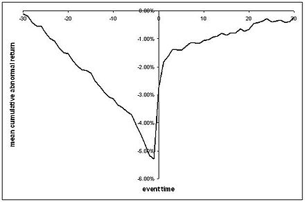
This regression allows you to talk about something similar to the kind of CAR series we usually see, where we have a plot of average abnormal returns before and after an event with maybe some standard errors around it:

(shamelessly taken from Wikipedia)

You'll need to come up with a distribution and error structure for the $e_{it}$'s,probably normally distributed, with some variance-co-variance structure. You can then set up a prior distribution for $\alpha_{i}$, $\beta_i$ and $\gamma_s$ and run Bayesian linear regression as was mentioned above.

Examining announcement effects

On the date of announcement it is reasonable to think there might be some abnormal returns ($\gamma_0\neq 0$). New information has just been released into the market, so reactions are not generally a violation of any kind of arbitrage or efficiency theorems. Neither you nor I know what announcement effects are likely to be. There isn't always much theoretical guidance either. So testing $\gamma_0=0$ may require much more specific knowledge than we have at our disposal (see below).

But part of the attraction of Bayesian analysis is that you can examine the entire posterior distribution of $\gamma_0$. This allows you to answer in some ways more interesting questions like "How likely is it that announcement excess returns are negative?" So for abnormal returns on the announcement date I would suggest abandoning strict hypothesis tests. You're not interested in them anyways - with most event studies you really want to know what the price reaction to an announcement may be, not what it is not!

In this vein one interesting summary of your posteriors might be the probability that $\gamma_0\geq 0$. Another could be the probability that $\gamma_0$ is higher than a variety of threshold values, or the quantiles of the posterior distribution for $\gamma_0$. Finally you can always plot the posterior of $\gamma_0$ along with it's mean, median and mode. But again strict hypothesis tests may not be what you want.

However for dates before and after the announcement, strict hypothesis testing can play an important role, because these returns can be viewed as tests of strong and semi-strong form efficiency

Testing for violations of semi-strong-form efficiency

Semi-strong-form effciency and an abscence of transaction costs imply that share prices should not continue to adjust after the announcment of the event. This corresponds to an intersection of sharp hypotheses that $\gamma_{s> 0}=0$.

Bayesians are uncomfortable with tests of this form, $\gamma_{s}=0$, called "sharp" tests. Why? Let's take this out of the context of finance for a second. If I asked you to form a prior over the average income of American citizens, $\bar x$ you would probably give me a continuous distribution, $f$ over possible incomes, maybe peaking around \$60,000. If you then took a sample of American incomes $X=\{x_i\}_{i=1}^n$ and tried to test the hypothesis that the population average was exactly $\$60,000$ you would use a Bayes factor:

$$P(\bar{x}=\$60,000|X)=\dfrac{\int_{\bar{x}=\$60,000} P(X) f(\bar{x})}{\int_{\bar{x}\neq \$60,000} P(X) f(\bar{x})}$$

The integral on top is zero, because the probability of a single point from the continuous prior distribution is zero. The integral on bottom would be 1, so $P(\bar{x}=\$60,000|X)=0$. This occurs because of the continuous prior, not because of anything essential to the nature of Bayesian inference.

In many ways tests that $\gamma_{s> 0}=0$ are asset pricing tests. Asset pricing is weird for Bayesians. Why is it weird? Because, in contrast to my prior over incomes, strict application of some efficiency hypotheses predicts an intercept of exactly 0 after the event. Any positive or negative $\gamma_{s>0}$ is a violation of semi-strong form efficiency, and potentially a huge profit making opportunity. So a valid prior could put positive probability on $\gamma_{s>0} =0$. This is exactly the approach taken in Harvey and Zhou (1990). More generally, imagine you have a prior with two parts. With probability $p$ you believe in strong-form efficiency ($\gamma_{s\neq 0} =0$) and with probability $1-p$ you don't believe in strong-form efficiency. Conditional on knowing strong-form efficiency is false, you think that there is a continuous distribution over $\gamma_{s>0}$, $f$. Then you can construct the Bayes factor test:

$$P(\gamma_{s> 0} =0|\text{data}) = \dfrac{P(\text{data}|\gamma_{s> 0}=0)p}{\int_{\gamma_{s> 0}\neq 0} P(\text{data}|\gamma_{s> 0})(1-p)f(\gamma_{s> 0})}>0$$

This test works because conditional on strong-form being true you would know that $\gamma_{s>0}=0$. In this case your prior is now a mixture of continuous and discrete distributions.

That a sharp test exists does not preclude you using more subtle tests. There is no reason you cannot examine the distribution of $\gamma_{s> 0}$ the same way I suggested for $\gamma_{s=0}$. This may be more interesting, especially since it is not dependent on a belief that transaction costs are non-existent. Credibile intervals could be formed, and based on your beliefs about transaction costs you could construct model tests based on intervals $\gamma_{s>0}$. Following Brav (2000) you could also predictive densities based on the "normal" return model ($\gamma_s=0$) to compare with actual returns, as a bridge between Bayesian and frequentist methods.

Cumulative abnormal returns

Everything so far has been a discussion of abnormal returns. So I'm going to go quickly into CAR:

$$\text{CAR}_\tau=\sum_{t=0}^\tau \gamma_{t}$$

This is a close counterpart to the average cumulative abnormal returns based on residuals that you are used to. You can find the posterior distribution using either numerical or analytic integration, depending on your prior. Because there is no reason to assume $\gamma_0=0$, there is no reason to assume $\text{CAR}_{t>0}=0$, so I would advocate the same analysis as with announcement effects, with no sharp hypothesis testing.

How to implement in Matlab

For a simple version of these models, you just need regular old Bayesian linear regression. I don't use Matlab but it looks like there's a version here. It's likely this works only with conjugate priors.

For more complicated versions, for instance the sharp hypothesis test, you will likely need a Gibbs sampler. I'm not aware of any out-of-the box solutions for Matlab. You can check for interfaces to JAGS or BUGS.