How to estimate real series from smoothed moving average?

Question

Suppose I have an observed time series $y_t$, which I suspect has been smoothed out. It appears to be significant autocorrelation at lag 1 and 2, therefore I suppose that the observed series $y_t$ is in the form:

$$y_t = \theta_0 x_t + \theta_1 x_{t-1} + (1 - \theta_0 - \theta_1)x_{t-2}$$

where $x_t$ is the original series I am after.

How can I recover the "original" series $x_t$? Clearly I need a method to estimate $\theta_0$ and $\theta_1$ and then apply the relevant transformation. But how to do that? I don't see how to apply an arima process here.

Answer 1

Your model can be written as arima model, or to be precise MA(2) model:

$$y_t= z_t+\alpha_1 z_{t-1}+\alpha_2 z_{t-2},$$

ARIMA models are usualy postulated with coefficient $1$ for $z_t$, because you can always move the multiplicative constant to the variance of the disturbances.

So your model

$$y_t= \theta_0x_t+\theta_1 x_{t-1}+(1-\theta_0-\theta_1) x_{t-2}$$

becomes MA(2) model

$$y_t= z_t+\frac{\theta_1}{\theta_0} z_{t-1}+\frac{1-\theta_0-\theta_1}{\theta_0} z_{t-2}$$

with $z_t=\theta_0x_t$.

So you can estimate MA(2) model and then recover $\theta_0$ and $\theta_1$ from $\alpha_1$ and $\alpha_2$:

$$\theta_0=\frac{1}{1+\alpha_1+\alpha_2},\quad \theta_1=\frac{\alpha_1}{1+\alpha_1+\alpha_2}$$

Here is the example in R:

set.seed(1001)
x<-rnorm(10000)
y<-filter(x,c(0.5,0.3,0.2),sides=1)
mod<-arima(y,order=c(0,0,2),include.mean=FALSE)
> mod
Call:
arima(x = y, order = c(0, 0, 2), include.mean = FALSE)

Coefficients:
         ma1     ma2
      0.6060  0.3874
s.e.  0.0093  0.0093

sigma^2 estimated as 0.2495:  log likelihood = -7246.14,  aic = 14498.28
> cf <- coef(mod) 
> 1/(1+sum(cf))
[1] 0.500497
> cf[1]/(1+sum(cf))
      ma1 
0.3007687 

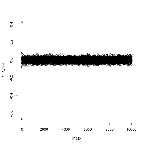
You can recover $x_t$ as residuals of the arima model:

x_rec<- as.numeric(residuals(mod)*(1+sum(cf)))
plot(x-x_rec)

As you see the procedure recovered coefficients with the precision of 3 decimal places. The recovered $x_t$ is also recovered to similar precision. The difference is the initialisation. ARIMA model assumes that the process is infinite, but the data is never infinite, so each estimation procedure must assume some initialisation. As evidenced from the plot the first few elements of recovered $x_t$ have the biggest error, but then the error stabilizes.

Since ARIMA models are estimated via Kalman filter procedure, you could implement it yourself with the proper intialisation. Note that in this example I used quite a big sample of 10000 elements. Less data would result in worse precision, you should run some tests to see the extent of the impact of sample size to the precision of recovery.

Answer 2

You can start with assuming that your observed variable is obtained from the true value as $$y_t = \theta_0 x_t + \theta_1 x_{t-1} + e_t$$

It would help to know what is the process of the underlying variable, suppose it's $$x_t = \beta_0 + \beta_1 x_{t-1} + u_t$$

where $e_t,u_t$ are errors. If these equations make sense to you then, you can estimate them using Kalman filter, see example here.

Next, you test whether $\theta_0+\theta_1=1$, if it holds statistically, then maybe your specification holds, so you can proceed with a constrained fit.

You have to set the expectations though: smoothing leads to data loss, generally. So, you can't reproduce the original series exactly. That's why using Kalman filter we had to make an assumption about the observed and true processes, i.e. we needed to inject some outside data to compensate for lost data (from smoothing) in order to recover the true series.