R-squared and fit of the model

Question

This post is new version of my last question. It was deleted due to my error in data. Currently data updated and verified. I have 2 models. Model 1 gives me:

Call:
lm(formula = A ~ B + C + D)

Residuals:
     Min       1Q   Median       3Q      Max 
-0.62281 -0.01037 -0.00011  0.01022  0.79359 

Coefficients:
               Estimate Std. Error t value Pr(>|t|)    
(Intercept)  -0.0002081  0.0001249  -1.667 0.095569 .  
B            -0.0136995  0.0040880  -3.351 0.000806 ***
C            -0.0115854  0.0044354  -2.612 0.009004 ** 
D             1.6885884  0.1038811  16.255  < 2e-16 ***
---
Signif. codes:  0 ‘***’ 0.001 ‘**’ 0.01 ‘*’ 0.05 ‘.’ 0.1 ‘ ’ 1

Residual standard error: 0.02495 on 39996 degrees of freedom
Multiple R-squared:  0.006786,  Adjusted R-squared:  0.006712 
F-statistic: 91.09 on 3 and 39996 DF,  p-value: < 2.2e-16

Model 2 gives me:

Call:
lm(formula = A ~ B)

Residuals:
     Min       1Q   Median       3Q      Max 
-0.62188 -0.01030 -0.00007  0.01019  0.79685 

Coefficients:
               Estimate Std. Error t value Pr(>|t|)   
(Intercept)  -0.0002189  0.0001252  -1.748  0.08047 . 
B            -0.0114271  0.0040951  -2.790  0.00527 **
---
Signif. codes:  0 ‘***’ 0.001 ‘**’ 0.01 ‘*’ 0.05 ‘.’ 0.1 ‘ ’ 1

Residual standard error: 0.02504 on 39998 degrees of freedom
Multiple R-squared:  0.0001946, Adjusted R-squared:  0.0001696 
F-statistic: 7.786 on 1 and 39998 DF,  p-value: 0.005266

Can someone explain me why Model 1 can be worse, then Model 2? I have only idea about miserable R-squared, which indicates that both models explain variation of dependent variable poorly. But nevertheless, I cant get, why model with more significant predictors and better R-squared can be worse.

Explanation of "worse". Both models predict some variable. Then this variable is checked against test sample (all other things - constant). Using MAE metrics I get better result for Model 2, than Model 1. I don't have access to test sample, only result of testing. I'm confused about it and looking for help, as, to my mind, there might be no situation where model 2 might be better.

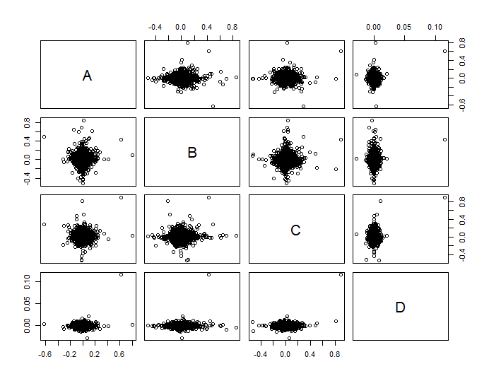
Scatter plot matrix ABCD, as asked below:

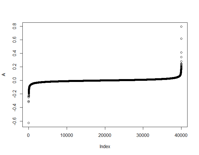
I believe that ascending plot of A might be helpful too:

Answer 1

The scatter plot matrix (and the quantile plot for A) indicate a family resemblance of all the variables, with

1. Both negative and positive values.

2. A strong concentration around a level of zero.

3. Some moderate outliers with absolute values around 0.5 to 1 or so.

This implies

• a possibility that the outliers might have undue influence on any regressions.

• an obligation to look inside the very dense cluster of points near zero, just in case there is some hidden structure. From the graphs, I am not hopeful, but we should look.

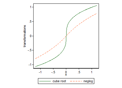
The idea of a transformation thus arises and it seems clear that an acceptable transformation must respect the sign of values and treat positive and negative tails similarly. That certainly rules out common fudges such as $\log(x + \text{fudge})$.

I suggested

cube root $x^{1/3}$

and @Flounderer suggested

$\text{sign}(x) \ln(1 + |x|)$, which has been dubbed the "neglog" transformation.

The data are not public, so only the OP can revisit the regressions using transformed scales to see if new ideas emerge. But the main point of this answer is to underline that for values like those in this dataset

• the neglog transformation is so close to linear that nothing much will change.

• the cube root is going to change distributions much more (and possibly relationships too).

Many readers will have a well-grounded intuition that logarithm-like transformations are much stronger than cube-root-like transformations, which is certainly correct for moderate or large values, but not in this case when we are so near the origin.

The graph here says it all:

As always, I stress that a transformation that seems a good idea as far as producing better behaved marginal distributions is concerned is not necessarily one that will produce clearer relationships between variables.

More on cube roots:

How to transform leptokurtic distribution to normality?

Regarding how to transform leptokurtic distribution to normality

More on neglog:

John, J.A. and N.R. Draper. 1980. An alternative family of transformations. Applied Statistics 29: 190-197.

Johnson, N.L. 1949. Systems of frequency curves generated by methods of translation. Biometrika 36: 149-176.

Whittaker, J., J. Whitehead and M. Somers. 2005. The neglog transformation and quantile regression for the analysis of a large credit scoring database. Applied Statistics 54: 863-878.

Answer 2

Here is an example of a fake data set which has the same sort of performance as your example:

set.seed(250116)
x3 <- rnorm(10000)
x1 <- rnorm(10000)
x2 <- rnorm(10000)
dat <- data.frame(x1, x2, x3, y = exp(5*x3) + rnorm(10000, 0, 0.1) + exp(4*(x1 + x2)))

model1 <- lm(y ~., data=dat[1:5000,])
model2 <- lm(y ~ x3, data=dat[1:5000,])

# dat[1:5000,] is the training data. The rest is test data.

mae1 <- sum(abs(predict(model1, dat[5001:10000, ]) - dat$y[5001:10000]))
    mae2 <- sum(abs(predict(model2, dat[5001:10000, ]) - dat$y[5001:10000]))

summary(model1)
summary(model2)
mae1
mae2

with the output:

> summary(model1)

Call:
lm(formula = y ~ ., data = dat[1:5000, ])

Residuals:
      Min        1Q    Median        3Q       Max 
 -1809596   -646466   -225528    216168 204514069 

Coefficients:
            Estimate Std. Error t value Pr(>|t|)    
(Intercept)   237539      76163   3.119  0.00183 ** 
x1            460482      76847   5.992 2.21e-09 ***
x2            390556      75730   5.157 2.60e-07 ***
x3            233292      77625   3.005  0.00267 ** 
---
Signif. codes:  0 ‘***’ 0.001 ‘**’ 0.01 ‘*’ 0.05 ‘.’ 0.1 ‘ ’ 1 

Residual standard error: 5385000 on 4996 degrees of freedom
Multiple R-squared: 0.01416,    Adjusted R-squared: 0.01357 
F-statistic: 23.92 on 3 and 4996 DF,  p-value: 2.309e-15 

> summary(model2)

Call:
lm(formula = y ~ x3, data = dat[1:5000, ])

Residuals:
      Min        1Q    Median        3Q       Max 
  -686743   -379900   -223291    -66778 206613240 

Coefficients:
            Estimate Std. Error t value Pr(>|t|)   
(Intercept)   231025      76619   3.015  0.00258 **
x3            233657      78094   2.992  0.00279 **
---
Signif. codes:  0 ‘***’ 0.001 ‘**’ 0.01 ‘*’ 0.05 ‘.’ 0.1 ‘ ’ 1 

Residual standard error: 5417000 on 4998 degrees of freedom
Multiple R-squared: 0.001788,   Adjusted R-squared: 0.001588 
F-statistic: 8.952 on 1 and 4998 DF,  p-value: 0.002785 

> mae1
[1] 4188685207
> mae2
[1] 2938392349

Here, model1 has more significant variables and a higher $R^2$, but model2 has lower mean absolute error on the test set.