27
$\begingroup$

I've heard/seen in several places that you can transform the data set into something that is normal-distributed by taking the logarithm of each sample, calculate the confidence interval for the transformed data, and transform the confidence interval back using the inverse operation (e.g. raise 10 to the power of the lower and upper bounds, respectively, for $\log_{10}$).

However, I'm a bit suspicious of this method, simply because it doesn't work for the mean itself: $10^{\operatorname{mean}(\log_{10}(X))} \ne \operatorname{mean}(X)$

What is the correct way to do this? If it doesn't work for the mean itself, how can it possibly work for the confidence interval for the mean?

$\endgroup$
3
  • 3
    $\begingroup$ You are quite right. This approach does not generally work and often yields confidence intervals that do not include the population mean or even the sample mean. Here is some discussion on it: amstat.org/publications/jse/v13n1/olsson.html This is not an answer, since I did not look into the matter enough to actually comment on the link in detail. $\endgroup$
    – Erik
    Commented Jul 31, 2012 at 8:53
  • 3
    $\begingroup$ This problem has a classic solution: projecteuclid.org/…. Some other solutions, including code, are provided at epa.gov/oswer/riskassessment/pdf/ucl.pdf--but read this with a heavy grain of salt, because at least one method described there (the "Chebyshev Inequality Method") is just plain wrong. $\endgroup$
    – whuber
    Commented Jul 31, 2012 at 15:21
  • $\begingroup$ @Erik. The URL you posted doesn't work. Here is a link that works (for me, now): jse.amstat.org/v13n1/olsson.html $\endgroup$ Commented Aug 27, 2022 at 18:18

7 Answers 7

19
$\begingroup$

There are several ways for calculating confidence intervals for the mean of a lognormal distribution. I am going to present two methods: Bootstrap and Profile likelihood. I will also present a discussion on the Jeffreys prior.

Bootstrap

For the MLE

In this case, the MLE of $(\mu,\sigma)$ for a sample $(x_1,...,x_n)$ are

$$\hat\mu= \dfrac{1}{n}\sum_{j=1}^n\log(x_j);\,\,\,\hat\sigma^2=\dfrac{1}{n}\sum_{j=1}^n(\log(x_j)-\hat\mu)^2.$$

Then, the MLE of the mean is $\hat\delta=\exp(\hat\mu+\hat\sigma^2/2)$. By resampling we can obtain a bootstrap sample of $\hat\delta$ and, using this, we can calculate several bootstrap confidence intervals. The following R codes shows how to obtain these.

rm(list=ls())
library(boot)

set.seed(1)

# Simulated data
data0 = exp(rnorm(100))

# Statistic (MLE)

mle = function(dat){
m = mean(log(dat))
s = mean((log(dat)-m)^2)
return(exp(m+s/2))
}

# Bootstrap
boots.out = boot(data=data0, statistic=function(d, ind){mle(d[ind])}, R = 10000)
plot(density(boots.out$t))

# 4 types of Bootstrap confidence intervals
boot.ci(boots.out, conf = 0.95, type = "all")

For the sample mean

Now, considering the estimator $\tilde{\delta}=\bar{x}$ instead of the MLE. Other type of estimators might be considered as well.

rm(list=ls())
library(boot)

set.seed(1)

# Simulated data
data0 = exp(rnorm(100))

# Statistic (MLE)

samp.mean = function(dat) return(mean(dat))

# Bootstrap
boots.out = boot(data=data0, statistic=function(d, ind){samp.mean(d[ind])}, R = 10000)
plot(density(boots.out$t))

# 4 types of Bootstrap confidence intervals
boot.ci(boots.out, conf = 0.95, type = "all")

Profile likelihood

For the definition of likelihood and profile likelihood functions, see. Using the invariance property of the likelihood we can reparameterise as follows $(\mu,\sigma)\rightarrow(\delta,\sigma)$, where $\delta=\exp(\mu+\sigma^2/2)$ and then calculate numerically the profile likelihood of $\delta$.

$$R_p(\delta)=\dfrac{\sup_{\sigma}{\mathcal L}(\delta,\sigma)}{\sup_{\delta,\sigma}{\mathcal L}(\delta,\sigma)}.$$

This function takes values in $(0,1]$; an interval of level $0.147$ has an approximate confidence of $95\%$. We are going to use this property for constructing a confidence interval for $\delta$. The following R codes shows how to obtain this interval.

set.seed(1)

# Simulated data
data0 = exp(rnorm(100))

# Log likelihood
ll = function(mu,sigma) return( sum(log(dlnorm(data0,mu,sigma))))

# Profile likelihood
Rp = function(delta){
temp = function(sigma) return( sum(log(dlnorm(data0,log(delta)-0.5*sigma^2,sigma)) ))
max=exp(optimize(temp,c(0.25,1.5),maximum=TRUE)$objective     -ll(mean(log(data0)),sqrt(mean((log(data0)-mean(log(data0)))^2))))
return(max)
}

vec = seq(1.2,2.5,0.001)
rvec = lapply(vec,Rp)
plot(vec,rvec,type="l")

# Profile confidence intervals
tr = function(delta) return(Rp(delta)-0.147)
c(uniroot(tr,c(1.2,1.6))$root,uniroot(tr,c(2,2.3))$root)

$\star$ Bayesian

In this section, an alternative algorithm, based on Metropolis-Hastings sampling and the use of the Jeffreys prior, for calculating a credibility interval for $\delta$ is presented.

Recall that the Jeffreys prior for $(\mu,\sigma)$ in a lognormal model is

$$\pi(\mu,\sigma)\propto \sigma^{-2},$$

and that this prior is invariant under reparameterisations. This prior is improper, but the posterior of the parameters is proper if the sample size $n\geq 2$. The following R code shows how to obtain a 95% credibility interval using this Bayesian model.

library(mcmc)

set.seed(1)

# Simulated data
data0 = exp(rnorm(100))

# Log posterior
lp = function(par){
if(par[2]>0) return( sum(log(dlnorm(data0,par[1],par[2]))) - 2*log(par[2]))
else return(-Inf)
}

# Metropolis-Hastings
NMH = 260000
out = metrop(lp, scale = 0.175, initial = c(0.1,0.8), nbatch = NMH)

#Acceptance rate
out$acc

deltap = exp(  out$batch[,1][seq(10000,NMH,25)] + 0.5*(out$batch[,2][seq(10000,NMH,25)])^2  )

plot(density(deltap))

# 95% credibility interval
c(quantile(deltap,0.025),quantile(deltap,0.975))

Note that they are very similar.

$\endgroup$
4
  • 1
    $\begingroup$ (+1) I think you can also get confidence intervals based on maximum-likelihood theory with the distrMod R package $\endgroup$ Commented Jul 31, 2012 at 11:51
  • $\begingroup$ @StéphaneLaurent Thanks for the info. I would like to see the outcome of your code with the new prior. I was not aware of the commands and the package that you are using. $\endgroup$
    – user10525
    Commented Jul 31, 2012 at 11:53
  • 5
    $\begingroup$ Beautiful response @Procrastinator. One other approach is the smearing estimator, which uses all the residuals off of the mean on the log scale to get $n$ predicted values on the original scale and simply averages them. I'm less up to date on confidence intervals using this approach though, except for using the standard bootstrap percentile method. $\endgroup$ Commented Jul 31, 2012 at 12:15
  • $\begingroup$ Superb response! The approaches suggested here assume homoscedastic model errors - I have worked on projects where this assumption was not tenable. I would also suggest the use of gamma regression as an alternative, which would bypass the need for a bias correction. $\endgroup$ Commented May 18, 2019 at 16:53
5
$\begingroup$

You might try the Bayesian approach with Jeffreys' prior. It should yield credibility intervals with a correct frequentist-matching property: the confidence level of the credibility interval is close to its credibility level.

 # required package
 library(bayesm)

 # simulated data
 mu <- 0
 sdv <- 1
 y <- exp(rnorm(1000, mean=mu, sd=sdv))

 # model matrix
 X <- model.matrix(log(y)~1)
 # prior parameters
 Theta0 <- c(0)
 A0 <- 0.0001*diag(1)
 nu0 <- 0 # Jeffreys prior for the normal model; set nu0 to 1 for the lognormal model
 sigam0sq <- 0
 # number of simulations
 n.sims <- 5000

 # run posterior simulations
 Data <- list(y=log(y),X=X)
 Prior <- list(betabar=Theta0, A=A0, nu=nu0, ssq=sigam0sq)
 Mcmc <- list(R=n.sims)
 bayesian.reg <- runireg(Data, Prior, Mcmc)
 mu.sims <- t(bayesian.reg$betadraw) # transpose of bayesian.reg$betadraw
 sigmasq.sims <- bayesian.reg$sigmasqdraw

 # posterior simulations of the mean of y: exp(mu+sigma²/2)
 lmean.sims <- exp(mu.sims+sigmasq.sims/2)

 # credibility interval about lmean:
 quantile(lmean.sims, probs = c(0.025, 0.975))
$\endgroup$
5
  • $\begingroup$ This sounds very interesting and since I tend to like Bayesian methods I upvoted it. It could still be improved by adding an some references or preferably even an understandable explanation on why it works. $\endgroup$
    – Erik
    Commented Jul 31, 2012 at 8:58
  • $\begingroup$ It is known that "it" (the frequentist-matching property) works for $\mu$ and $\sigma^2$. For $\mu$ the frequentist-matching property is perfect: the credibility interval is exactly the same as the usual confidence interval. For $\sigma^2$ I don't know whether it is exact but it is easy to check because the posterior distribution is an inverse-Gamma. The fact that it works for $\mu$ and $\sigma^2$ does not necessarily implies that it works for a function $f(\mu, \sigma^2)$ of $\mu$ and $\sigma^2$. I don't know whether there are some references but otherwise you can check with simulations. $\endgroup$ Commented Jul 31, 2012 at 9:17
  • $\begingroup$ Many thanks for the discussion. I deleted all my comments for clearness and to avoid any confusion. (+1) $\endgroup$
    – user10525
    Commented Jul 31, 2012 at 15:08
  • 1
    $\begingroup$ @Procrastinator Thanks too. I have also deleted my comments and added the point about the Jeffreys prior in my code. $\endgroup$ Commented Jul 31, 2012 at 15:15
  • $\begingroup$ Could someone please explain to me how boots.out = boot(data=data0, statistic=function(d, ind){mle(d[ind])}, R = 10000) works. I see that "ind" is an index, but I don't understand how to find "ind". Where is this second argument referencing? I've tried it with alternative functions and it did not work. Looking at the actual function boot, I don't see a reference to Ind either. $\endgroup$ Commented Sep 30, 2015 at 2:32
4
$\begingroup$

Another approximate confidence interval for the mean $\delta = \exp\left(\mu+\sigma^2/2\right)$ of the i.i.d. random variables in a random sample $\left(X_1, \ldots, X_n\right)$ of size $n$ from a $\mathcal{LN}\left(\mu,\sigma^2\right)$ distribution can be established by considering the asymptotic distribution of the MLE $\hat\delta = \exp\left(\hat\mu + \hat\sigma^2/2\right)$ for $\delta$, which can be obtained by applying the multivariate delta method to the asymptotic distribution of the MLE $\left(\hat\mu, \hat\sigma^2\right)^\top$ for $\left(\mu, \sigma^2\right)^\top$:
The entries of $\left(\hat\mu, \hat\sigma^2\right)^\top$ are given by $$ \hat\mu = \frac{1}{n} \sum_{i=1}^n\ln\left(x_i\right),\\ \hat\sigma^2 = \frac{1}{n} \sum_{i=1}^n\left(\ln\left(x_i\right)-\hat\mu\right)^2. $$ From MLE theory we know that $$ \sqrt{n} \left( \begin{pmatrix} \hat\mu \\ \hat\sigma^2 \end{pmatrix} - \begin{pmatrix} \mu \\ \sigma^2 \end{pmatrix} \right) \overset{d}{\to} \mathcal N\left( \begin{pmatrix} 0 \\ 0 \end{pmatrix}, I\left(\mu, \sigma^2\right)^{-1} \right), $$ where $I\left(\mu, \sigma^2\right)^{-1} = \mathrm{diag}\left( \sigma^2, 2\sigma^4 \right)$ is the inverse of the expected Fisher information from a single $X_i$.$^\star$
The gradient of $\left(\mu, \sigma^2\right) \mapsto \exp\left(\mu+\sigma^2/2\right)$ is given by $\left(\exp\left(\mu+\sigma^2/2\right), \exp\left(\mu+\sigma^2/2\right)/2\right)^\top$ and hence the delta method yields $$ \sqrt{n} \left(\hat\delta - \delta\right) \overset{d}{\to} \mathcal{N}\left(0, \delta^2 \sigma^2 \left(1+\frac{\sigma^2}{2} \right) \right). $$
Finally, after replacing $\delta^2$ and $\sigma^2$ with its consistent estimators $\hat\delta^2$ and $\hat\sigma^2$, we get the approximate $(1-\alpha)\times 100\%$ confidence interval $$ \hat\delta \mp z_{1-\alpha/2} \times \hat\delta \times \frac{1}{\sqrt n} \times \sqrt{\hat\sigma^2\left(1+\frac{\hat\sigma^2}{2}\right)} $$ for $\delta$.

alpha <- 0.05
n <- 100
mu <- 0
sigma_sq <- 1

x <- rlnorm(n, mu, sqrt(sigma_sq))

mu_mle <- mean(log(x)) 
sigma_sq_mle <- mean((log(x) - mu_mle)^2)
delta_mle <- exp(mu_mle + sigma_sq_mle/2)
z <- qnorm(1 - alpha/2)
moe <- z * delta_mle * 1/sqrt(n) * sqrt(sigma_sq_mle * (1 + sigma_sq_mle/2))

sprintf("%d%% CI for the mean: [%f, %f]",
       (1-alpha)*100, delta_mle - moe, delta_mle + moe)

$^\star$This seems to be wrong in the Wikipedia article on the log-normal distribution (accessed 2022-08-28).

$\endgroup$
3
$\begingroup$

Ulf Olsson (2005)$^{[1]}$ presents several possibilities of calculating confidence intervals for a lognormal mean. First, let's clarify the notation. Let $X$ be a random variable following a log-normal distribution with mean $\operatorname{E}(X)=\theta$. Let $Y = \log(X)$ be the log-transformed variable which is normally distributed with mean $\operatorname{E}(Y)=\mu$ and variance $\operatorname{Var}(Y)=\sigma^2$. The sample equivalents of the mean and variance of $Y$ are $\bar{y}$ and $s^2$. We seek a confidence interval for the mean of $X$, defined as $$ \operatorname{E}(X) = \theta = e^{\left(\mu + \frac{\sigma^2}{2}\right)} $$ A possible $(1 - \alpha)\,\%$-confidence interval for $\log(\theta)$ is given by (see also Zhou et al. 1997$^{[2]}$): $$ \bar{y}+\frac{s^2}{2}\pm z_{1-\alpha/2}\sqrt{\frac{s^2}{n}+\frac{s^4}{2(n-1)}} $$ where $z_{1-\alpha/2}$ is the appropriate quantile of the standard normal distribution. The limits of this confidence interval are then back-transformed to give a confidence interval for $\theta$.

Olsson recommends using $t$-quantiles with $n-1$ degrees of freedom instead of $z$-quantiles: $$ \bar{y}+\frac{s^2}{2}\pm t_{1-\alpha/2, n-1}\sqrt{\frac{s^2}{n}+\frac{s^4}{2(n-1)}} $$

He found that this modification improved the performance, although the coverage probability was lower than nominal for $n<50$.

Let's inspect the performance of this formula in a very small simulation:

# The function to calculate the CI
ci_lnorm <- function(x, alpha = 0.05) {
  n <- length(x)
  tval <- qt(1 - alpha/2, n - 1)
  y <- log(x)
  ybar <- mean(y)
  s <- sd(y)
  exp(ybar + s^2/2 + c(-1, 1)*tval*sqrt((s^2/n) + (s^4/(2*(n - 1)))))
}

# True parameters of X (on normal log-scale)
mu <- 1
s <- 2.5

true_mean <- exp(mu + (1/2)*s^2)

# Simulation

set.seed(142857)
res <- replicate(1e5, {
  x <- rlnorm(10, mu, s)
  ci <- ci_lnorm(x)
  ifelse(ci[2] > true_mean && ci[1] < true_mean, 1, 0)
})

# Coverage
mean(res)
[1] 0.91053

The simulated coverage for $n=10, \mu = 1, \sigma = 2.5$ is around $91.1\,\%$ based on $100\,000$ simulations.

References

$[1]:$ Olsson, U. (2005). Confidence intervals for the mean of a log-normal distribution. Journal of Statistics Education, 13(1). (link)

$[2]:$ Zhou, X. H., & Gao, S. (1997). Confidence intervals for the log‐normal mean. Statistics in medicine, 16(7), 783-790. (link)

$\endgroup$
2
$\begingroup$

However, I'm a bit suspicious of this method, simply because it doesn't work for the mean itself: 10mean(log10(X))≠mean(X)

You're right -- that's the formula for the geometric mean, not the arithmetic mean. The arithmetic mean is a parameter from the normal distribution, and is often not very meaningful for lognormal data. The geometric mean is the corresponding parameter from the lognormal distribution if you want to talk more meaningfully about a central tendency for your data.

And you would indeed calculate the CIs about the geometric mean by taking the logarithms of the data, calculating the mean and CIs as usual, and back-transforming. You're right that you really don't want to mix your distributions by putting the CIs for the geometric mean around the arithmetic mean....yeowch!

$\endgroup$
2
$\begingroup$

As @dnidz said, you probably want to be computing the geometric mean and its CI, not the arithmetic mean and its CI, when data are sampled from a lognormal distribution. Why?

First, let's think about normal distributions. For an ideal normal population (distribution), the arithmetic mean and the median are identical. For any given sample, those two values are usually not identical. Which of the two values is likely to be closer to the true mean (and median; they are the same) of the population? The median is computed only from the ranks of the values. The arithmetic mean is computed from the actual values and takes into account an assumption about the distribution. If that assumption of sampling from a normal assumption is true, the arithmetic mean of the sample is likely to be closer to the mean and median of the distribution than is the median of the sample. That is why the arithmetic mean (the average) is so commonly used.

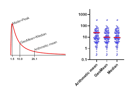
Now let’s switch to the lognormal distribution. The median and geometric mean of an ideal lognormal distribution are identical, but the arithmetic mean has a larger value. How much larger depends on how asymmetrical the distribution is as expressed by the Geometric standard deviation. Your goal (I assume) is to estimate the median of the population (or distribution) from a sample of data. If you are sampling from a lognormal population, the best estimate is the geometric mean. That is likely to be a better estimate than the sample median and a much better estimate than the arithmetic mean.

The figure on the left below shows an ideal lognormal distribution (GeoMean=10; GeoSD=4) with its arithmetic and geometric mean. The graph on the right shows a sample of data (on a logarithmic axis) showing the two means and the median.

enter image description here

If you agree that the geometric mean is most appropriate:

  1. Transform all values to logarithms.
  2. Compute the arithmetic mean and the 95% CI of that mean from the set of logarithms.
  3. Back transform the mean and both confidence limits to the original units. You'll have calculated the geometric mean and its 95% CI. (Biologists use the common base 10 logarithm and the 10^ back transofrm. Mathematicians and physical scientists use the natural ln logarithm and the exp() back transform. The results will be the same either way.)
$\endgroup$
1
$\begingroup$

On R you can try EnvStats::elnorm(data_vector, ci = TRUE)$interval$limits

Otherwise, on the below answer you can see how to get either prediction on confidence intervals with different prob values.

https://stats.stackexchange.com/a/109236/162190

Both ways give the same limits of CI.

$\endgroup$

Your Answer

By clicking “Post Your Answer”, you agree to our terms of service and acknowledge you have read our privacy policy.

Not the answer you're looking for? Browse other questions tagged or ask your own question.