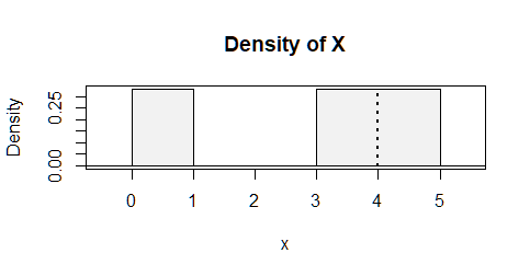
Let's approximate the probability of interest $P\left(\sum_{i = 1}^{1296}X_i \leq 3600\right)$ in two ways to verify if the CLT approximation is reliable for this specific problem.
CLT Approximation
As usual, denote the i.i.d. sum $X_1 + X_2 + \cdots + X_n$ by $S_n$. Using the moments calculated in whuber's answer, the classical CLT tells us
\begin{align*}
\frac{S_n - \frac{17}{6}n}{\sqrt{\frac{107}{36}n}} \to_d Z \sim N(0, 1). \tag{1}\label{1}
\end{align*}
According to $\eqref{1}$, $P\left(\sum_{i = 1}^{1296}X_i \leq 3600\right)$ can be evaluated as follows:
\begin{align*}
& P\left(\sum_{i = 1}^{1296}X_i \leq 3600\right) \\
=& P(S_{1296} \leq 3600) \\
=& P\left(\frac{S_{1296} - \frac{17}{6} \times 1296}{\sqrt{\frac{107}{36} \times 1296}}\leq
\frac{3600 - \frac{17}{6} \times 1296}{\sqrt{\frac{107}{36} \times 1296}} \right) \\
\approx & P(Z \leq -1.160084) \\
=& \Phi(-1.160084) = 0.1230073. \tag{2}\label{2}
\end{align*}
Monte Carlo Simulation
To validate if $\eqref{2}$ is a good approximation, let's simulate $N$ samples
$$\mathcal{S}_i = \{X_1^{(i)}, \ldots, X_{1296}^{(i)}\}, i = 1, \ldots, N$$
from density $f$ directly, and use the proportion $\frac{1}{N}\sum_{i = 1}^N I\left(X_1^{(i)} + \ldots + X_{1296}^{(i)} \leq 3600\right)$ to approximate $P\left(\sum_{i = 1}^{1296}X_i \leq 3600\right)$. The R code and results are as follows:
N <- 100000
S <- matrix(sample(c(0, 3, 4), size = N * 1296, replace = TRUE) + runif(N * 1296),
            nrow = N, ncol = 1296)
iidSum <- rowSums(S)
mean(iidSum <= 3600)
#  0.1221
The Monte Carlo estimate 0.1221 (your run may be different from mine for different random seeds) shows that the CLT approximation 0.1230073 is quite accurate.
Rejoinder to Concerns/Warnings in Comments
Under the original post, @Frank Harrell commented:
(to OP)Your instructor made a possibly ill-posed question because the CLT may not apply with that sample size, depending on the level of accuracy you need from a CLT approximation. n=1296 is not necessarily large at all.
(to me) You’re making the common mistake of assuming that a limit theorem applies to practical problems.
I found these comments are off-topic/irrelevant to this very well-posed problem.
First of all, this question itself is purely probabilistic (i.e., mathematical), not statistical: the question gives a density $f$ with finite variance and asks to approximate the quantity $p := P\left(\sum_{i = 1}^{1296}X_i \leq 3600\right)$ using CLT, provided that $X_1, \ldots, X_{1296} \text{ i.i.d} \sim f$, period. Here $X_1, \ldots, X_{1296}$ are hypothetical random variables instead of observed data. While it is reasonable to challenge whether the CLT approximation of $p$ is good enough (I will address this challenge shortly in the second bullet point later), I am completely baffled with the "ill-posed question" comment and "assuming the limiting theorem applies to practical problems" comment -- there is no "practical problems" under consideration at all and I didn't "assume" anything in my comment or solution.
Second, under the condition of the classical CLT, plus the finite third moment condition (which is clearly satisfied by the density $f$ in this question), the Berry-Essen Theorem guarantees that the error of the CLT approximation is bounded by a constant of order $\frac{1}{\sqrt{n}}$, more specifically,
\begin{align*}
\sup_{x \in \mathbb{R}^1}|F_n(x) - \Phi(x)| \leq \frac{C\rho}{\sqrt{n}\sigma^3},
\end{align*}
where $\rho = E[|X|^3]$ and $C < 0.4748$. For this problem, $\rho = \frac{545}{12}$, $\sigma = \sqrt{\frac{107}{36}}$, hence the worst error is at most
\begin{align*}
\frac{0.4748 \times \frac{545}{12}}{\sqrt{1296} \times \left(\frac{107}{36}\right)^{3/2}} \approx 0.12.
\end{align*}
Although $0.12$ is clearly too big for this particular problem, but do remember this is a uniform bound. At $x_0 = -1.160084$, according to the Edgeworth correction to the normal approximation (cf. Theorem 2.4.3 of Elements of Large Sample Theory by E. L. Lehmann) the difference between $F_n(x_0)$ and $\Phi(x_0)$ is of the order:
\begin{align*}
\frac{\mu_3}{6\sigma^3\sqrt{n}}(1 - x_0^2)\varphi(x_0) = 0.0001589854,
\end{align*}
which is very accurate. Therefore, it is confident to say that with $n = 1296$, the CLT approximation to $p$ does an "excellent job". Again, this is guaranteed by theory, which is indisputable by any empirical evidence or practical experience.
Third, rejoinder to the lognormal example. @Frank Harrell urged me to try out this example based on which he claimed " a log-normal distribution where $n=50,000$ is far too small to get accurate confidence intervals with CLT". After checking this example, I found the 95% confidence interval for $\theta = \exp(\mu + \sigma^2/2)$ with $X_1, \ldots, X_n \text{ i.i.d. } \sim LN(\mu, \sigma^2)$ in the link is formed as
\begin{align*}
\bar{X} \pm t_{n - 1}(0.025)\frac{\operatorname{sd}(X)}{\sqrt{n}}.
\end{align*}
Unfortunately, this is not the correct way of applying CLT to construct CI: forming a confidence interval following the vanilla recipe "sample mean $\pm$ multiplier $\times$ standard error" is NOT equivalent to "applying CLT correctly to construct a confidence interval". In this case, the correct confidence interval for $\theta$ that is based on a correct application of the (multivariate) CLT can be found in this answer by statmerkur:
\begin{align*}
\hat\delta \mp z_{1-\alpha/2} \times \hat\delta \times \frac{1}{\sqrt n} \times \sqrt{\hat\sigma^2\left(1+\frac{\hat\sigma^2}{2}\right)}.
\end{align*}
See the linked post for notation definitions in the above expression. With this CI and $n = 50,000$, the coverage probability is very close to the desired confidence level 95%:
alpha <- 0.05
n <- 50000
mu <- 0
sigma_sq <- 1
theta = exp(mu + sigma_sq/2) # True mean

N <- 1000 # Number of simulation replicates
out <- rep(0, N)

for (i in 1:N) {
  x <- rlnorm(n, mu, sqrt(sigma_sq))
  mu_mle <- mean(log(x))
  sigma_sq_mle <- mean((log(x) - mu_mle)^2)
  delta_mle <- exp(mu_mle + sigma_sq_mle/2)
  z <- qnorm(1 - alpha/2)
  moe <- z * delta_mle * 1/sqrt(n) * sqrt(sigma_sq_mle * (1 + sigma_sq_mle/2))
  out[i] <- (theta >= delta_mle - moe) & (theta <= delta_mle + moe)
}

mean(out)
# 0.952
To conclude, there is nothing (and cannot be) wrong about CLT when the conditions (i.i.d., finite second moment) are all met (after all, it is the culminating theorem in probability theory). But people who tried to apply it should exercise caution to avoid any misuse.

