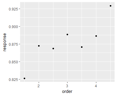
I fitted a glmer model to my data in r (with package lme4), one of significant fixed effects (order, which is continuous) has a negative estimate. But when I graph the averaged data, it seems to have a positive slope. what is going on here?
My response variable is binary. Here is my model:
g2amin = glmer (response ~ WMC + order + distance + DomSide + BlockType + (1 | pno) + WMC:order + WMC:distance + WMC:DomSide + order:DomSide + distance:DomSide + WMC:BlockType + distance:BlockType + DomSide:BlockType + order:BlockType, data = StudyDataN[StudyDataN$group == "Depressed",], family = binomial(link = "logit"))
And here is the summary of a results:
    > summary(g2amin)

 Generalized linear mixed model fit by maximum likelihood (Laplace Approximation) [glmerMod]
 Family: binomial  ( logit )
Formula: response ~ WMC + order + distance + DomSide + (1 | pno) + BlockType +
    WMC:order + WMC:distance + WMC:DomSide + order:DomSide +
    distance:DomSide + WMC:BlockType + distance:BlockType + DomSide:BlockType +
    order:BlockType
   Data: StudyDataN[StudyDataN$group == "Depressed", ]

     AIC      BIC   logLik deviance df.resid
  1667.7   1809.7   -809.9   1619.7     2716

Scaled residuals:
    Min      1Q  Median      3Q     Max
-9.0582  0.1218  0.1916  0.3408  1.4150

Random effects:
 Groups Name        Variance Std.Dev.
 pno    (Intercept) 1.533    1.238
Number of obs: 2740, groups:  pno, 35

Fixed effects:
                                     Estimate Std. Error z value Pr(>|z|)
(Intercept)                         0.1868731  0.8957168   0.209  0.83474
WMC                                 0.4359188  0.1643682   2.652  0.00800 **
order                              -0.0552924  0.1989800  -0.278  0.78111
distance2                          -0.0764481  0.4146961  -0.184  0.85374
distance3                           0.6319618  0.4773702   1.324  0.18556
distance4                           0.3508307  0.6401691   0.548  0.58367
DomSideRightDominant               -0.3313894  0.5686869  -0.583  0.56008
BlockTypeEasy                      -0.5018924  0.5723332  -0.877  0.38053
WMC:order                          -0.0003284  0.0360465  -0.009  0.99273
WMC:distance2                      -0.0011375  0.0751027  -0.015  0.98792
WMC:distance3                      -0.0112596  0.0861449  -0.131  0.89601
WMC:distance4                      -0.0105631  0.1175462  -0.090  0.92840
WMC:DomSideRightDominant           -0.0339368  0.0626720  -0.541  0.58816
order:DomSideRightDominant          0.1314148  0.1486902   0.884  0.37680
distance2:DomSideRightDominant      0.2820502  0.3102362   0.909  0.36327
distance3:DomSideRightDominant     -0.1464505  0.3594309  -0.407  0.68368
distance4:DomSideRightDominant     -0.0905467  0.4886552  -0.185  0.85300
WMC:BlockTypeEasy                  -0.0997565  0.0652019  -1.530  0.12603
distance2:BlockTypeEasy             0.2922394  0.3161517   0.924  0.35530
distance3:BlockTypeEasy            -0.4349740  0.3613730  -1.204  0.22872
distance4:BlockTypeEasy             0.4364490  0.5110543   0.854  0.39310
DomSideRightDominant:BlockTypeEasy  0.1938680  0.2662980   0.728  0.46661
order:BlockTypeEasy                 0.5382489  0.1523153   3.534  0.00041 ***
---
Signif. codes:  0 ‘***’ 0.001 ‘**’ 0.01 ‘*’ 0.05 ‘.’ 0.1 ‘ ’ 1

Correlation matrix not shown by default, as p = 23 > 12.
Use print(x, correlation=TRUE)  or
     vcov(x)     if you need it

convergence code: 0
Model failed to converge with max|grad| = 0.00838529 (tol = 0.001, component 1)
I checked chi-square statistic to see which fixed effects are significant (using package car)
 > Anova(g2amin)
Analysis of Deviance Table (Type II Wald chisquare tests)

Response: response
                     Chisq Df Pr(>Chisq)
WMC                10.8837  1  0.0009701 ***
order               9.0390  1  0.0026427 **
distance            4.6383  3  0.2002791
DomSide             0.0630  1  0.8017518
BlockType          28.4340  1  9.695e-08 ***
WMC:order           0.0001  1  0.9927304
WMC:distance        0.0230  3  0.9990761
WMC:DomSide         0.2932  1  0.5881645
order:DomSide       0.7811  1  0.3767953
distance:DomSide    1.5261  3  0.6762667
WMC:BlockType       2.3408  1  0.1260258
distance:BlockType  4.3078  3  0.2300926
DomSide:BlockType   0.5300  1  0.4666066
order:BlockType    12.4876  1  0.0004097 ***
---
Signif. codes:  0 ‘***’ 0.001 ‘**’ 0.01 ‘*’ 0.05 ‘.’ 0.1 ‘ ’ 1
and variable order is significant in my model. Here is a graph of averaged data over the other variables (BlockType, distance, ...):

order's slope in graph is obviously positive, but why it's negative in my model? Is the whole point of graphing for binomial data wrong??
