You don't want to fix the smoothness parameters at some values. What you want to do is to try to control the behaviour of the spline at locations beyond the data.
Wood (2016) sets out one way to achieve this. The general idea is to place most of the knots for the spline within the limits of the data, but to place outer and inner boundary knots to bracket the region where you want the penalty to operate over but where you have no data.
Simon shows how to do this in the 1-d case, where he places knots specifically
b <- gam(y ~ s(x, bs = "bs", m = c(3,1), k = 20),
         knots = list(x = c(-.5,0,1,1.5)),
         method = "ML")
which has a second order penalty (implied by the c(3,1) passed to m), outer knots at -0.5 and 1.5, inner knots and 0 and 1, and then remaining knots (implied) spread evenly over the range 0–1.
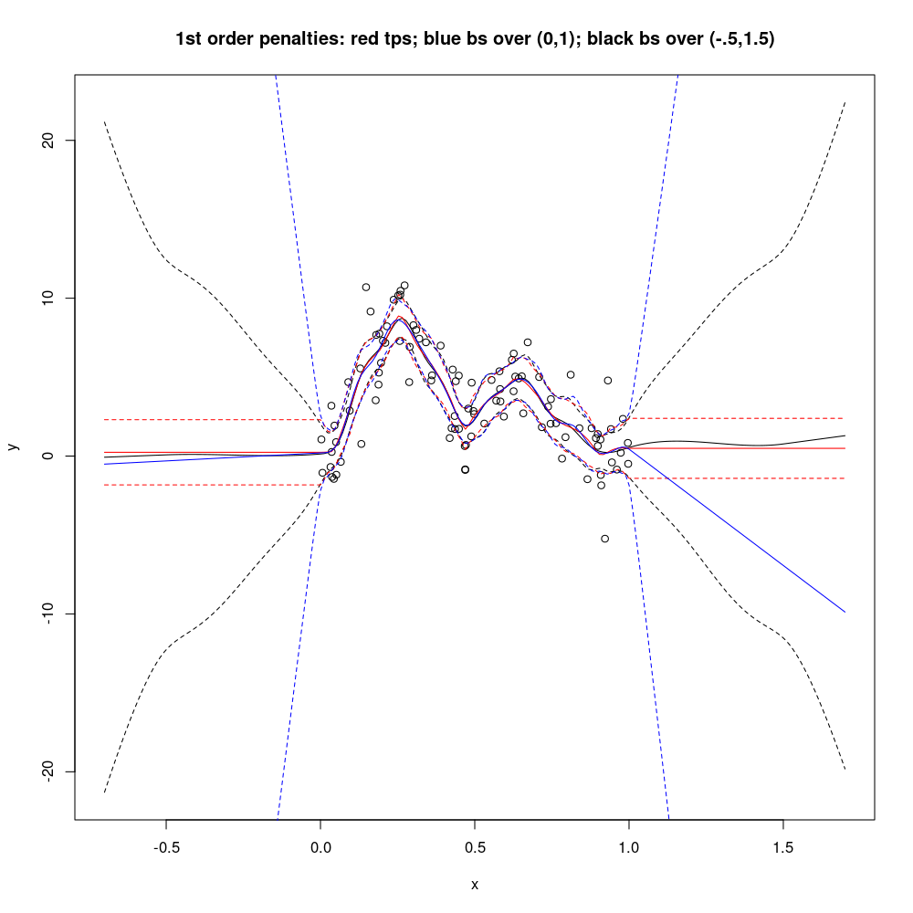
The full example in ?smooth.construct.bs.smooth.spec produces the following plot (code from the example shown below)

The red line is the result of a thin plate spline with penalty on the first derivative. The CI is constant because the slope of the line must be linear otherwise the penalty explodes to infinity. The constant CI is not a good description of our uncertainty as we extrapolate however; we would expect uncertainty to increase as we move further from the support of the data.
The blue line shows what happens in the usual case where knots are restricted to the range of the data and we use a b spline with second derivative penalty. The CI explodes because there is no penalty outside the range of the data.
The black line shows the effect of pushing the penalty out to -0.5 and 1.5. Because the penalty acts beyond the range of the data the CI is constrained. Notice however that in the example Simon has predicted a little bit beyond the limits of the region where the penalty applies; -0.7--1.7. This accounts for the change in the rate of increase in the spread of the CI. It explodes quickly again once the penalty is turned off beyond the specified interval -0.5--1.5.
So, in your example you want to follow the same idea, to set inner knots covering the range of the data in the two coordinates, and then add outer boundary knots to cover the interval you want to extrapolate over.
Code for the example. All from ?smooth.construct.bs.smooth.spec
f3 <- function(x) 0.2 * x^11 * (10 * (1 - x))^6 + 10 * (10 * x)^3 * (1 - x)^10 ## test function
n <- 100
x <- runif(n)
y <- f3(x) + rnorm(n)*2

## first a model with first order penalty over whole real line (red)
b0 <- gam(y~s(x,m=1,k=20),method="ML")

## now a model with first order penalty evaluated over (-.5,1.5) (black)
b <- gam(y~s(x,bs="bs",m=c(3,1),k=20),knots=list(x=c(-.5,0,1,1.5)),
         method="ML")

## and the equivalent with same penalty over data range only (blue)
b1 <- gam(y~s(x,bs="bs",m=c(3,1),k=20),method="ML")

## predict at new data extrapolating
pd <- data.frame(x=seq(-.7,1.7,length=200))

## fitted values for model `b` - the black line in the plot
fv <- predict(b,pd,se=TRUE)
## create a confidence band for the original fit, upper first, then lower
ul <- fv$fit + fv$se.fit*2
ll <- fv$fit - fv$se.fit*2

plot(x,y,xlim=c(-.7,1.7),ylim=range(c(y,ll,ul)),
     main= "1st order penalties: red tps; blue bs over (0,1); black bs over (-.5,1.5)")
lines(pd$x,fv$fit)
lines(pd$x,ul,lty=2)
lines(pd$x,ll,lty=2)

## fitted values and CI for the b0 model, red line
fv <- predict(b0,pd,se=TRUE)
ul <- fv$fit + fv$se.fit*2
ll <- fv$fit - fv$se.fit*2

## penalty defined on whole real line gives constant width intervals away
## from data, as slope there must be zero, to avoid infinite penalty:
lines(pd$x,fv$fit,col=2)
lines(pd$x,ul,lty=2,col=2)
lines(pd$x,ll,lty=2,col=2)

## fitted values for the b1 model, where penalty is only over the
## range of the data, blue line
fv <- predict(b1,pd,se=TRUE)
ul <- fv$fit + fv$se.fit*2
ll <- fv$fit - fv$se.fit*2

## penalty defined only over the data interval (0,1) gives wild and wide
## extrapolation since penalty has been `turned off' outside data range:
lines(pd$x,fv$fit,col=4)
lines(pd$x,ul,lty=2,col=4)
lines(pd$x,ll,lty=2,col=4)
Wood, S. N. 2016. P-splines with derivative based penalties and tensor product smoothing of unevenly distributed data. Stat. Comput. 1–5. doi:10.1007/s11222-016-9666-x
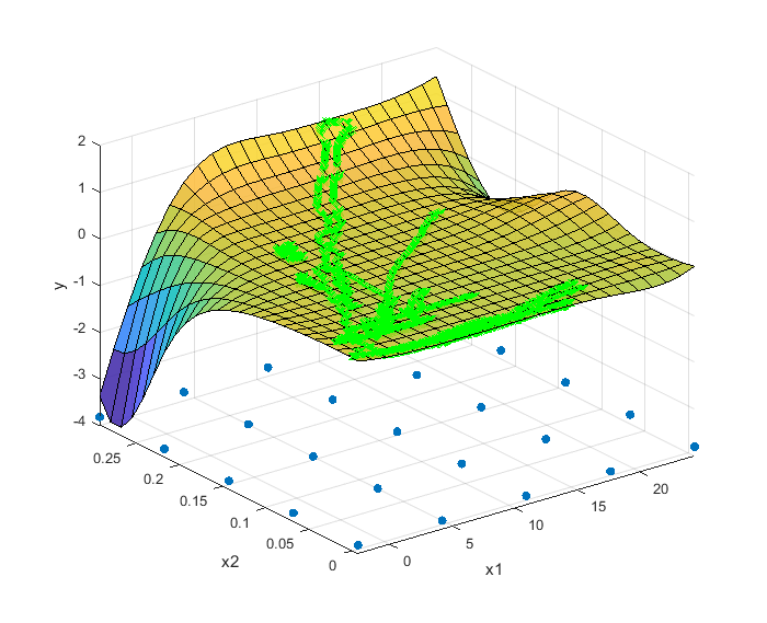
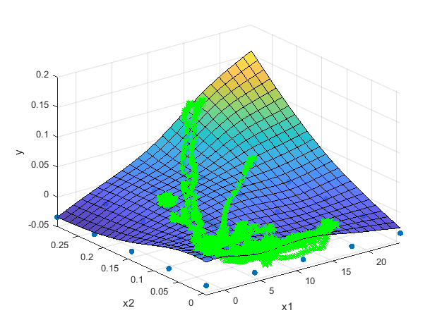
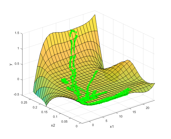 which shows that I have a nice match where the function is supported by data. But in areas where there is no data to support the function, the model is a bit wild.