Standardise distance to the mean of normal distribution
In my understanding, Z-score and Mahalanobis distance are the standardising methods to measure the closeness to the mean of a distribution, where we need to consider the direction and variance of the dispersions.
Question
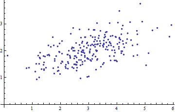
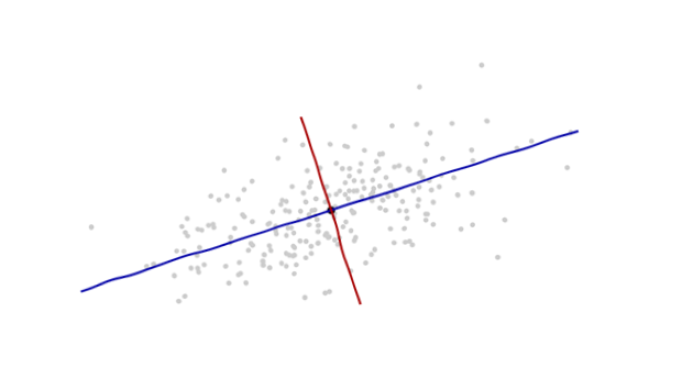
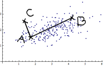
Which one, A or B, is closer to the mean of the distribution, or conversely which is more remote outlier to the distribution.

Direction and variance of the dispersions
To answer the question, I need to consider the direction and variance of the dispersions in the distribution.
Although the visible distances to A and B look similar, B belongs to the distribution and A is an outlier. The distance to the mean should be shorter (closer to the mean) along the direction to B with the larger dispersion (higher variance).
(Direction, Variance) to (Eigenvector, Eigenvalue)
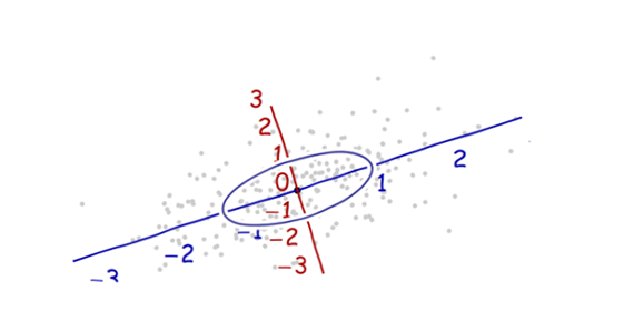
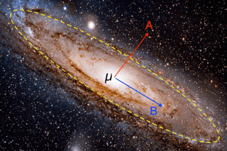
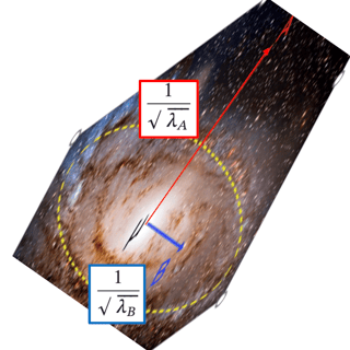
The eigenvectors $u_i$ tell the directions of the dispersions, and the eigenvalues $\lambda_i$ tell the variances of the dispersions. Higher eigenvalue means larger variance. Then if I scale the space by $\frac {1}{\sqrt{\lambda_A}}$ in the A direction and
$\frac {1}{\sqrt{\lambda_B}}$ in the B direction, I can decide which is close to the mean by comparing:
$$\frac {\Vert A-\mu \Vert}{\sqrt{\lambda_A}} \text {and} \frac {\Vert B-\mu \Vert}{\sqrt{\lambda_B}}$$
The distance in the direction with higher variance gets shorter.

Standardise distance to mean
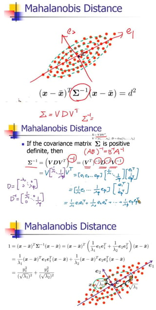
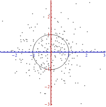
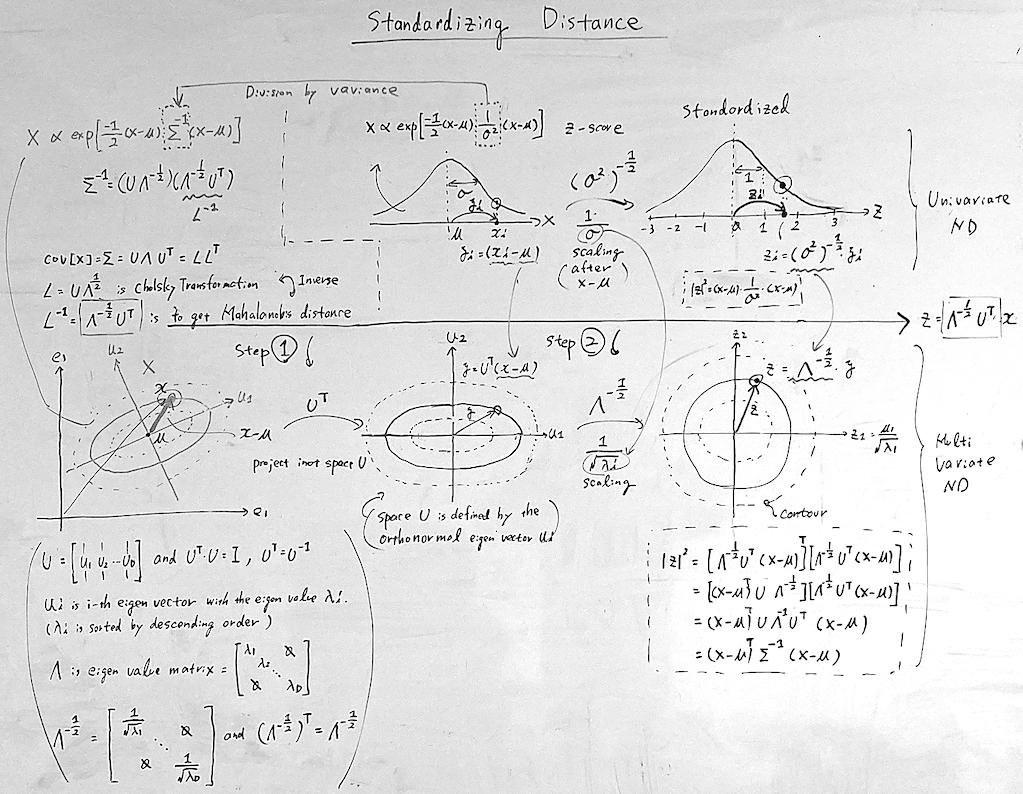
In a univariate normal distribution where there is only one direction of dispersion and one variance $\sigma^2$, I can standardise the distance via Z-score as in the top half of the snapshot.
In multivariate normal distribution, I can standardise the distance as in the bottom of the snapshot via the steps:
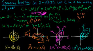
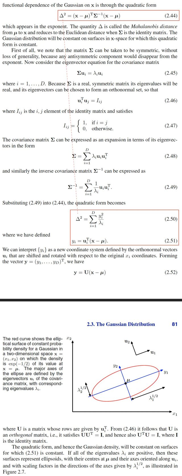
- Project $(X - \mu)$ into the U space where the unit eigenvectors $u_i$ are the orthonormal axes. This operation is changing the coordinate in X space to the coordinate in U space.
- Scale to the $u_i$ directions by $$\frac {1}{\sqrt{\lambda_i}}$$ where $\lambda_i$ is the eigenvalues for the eigenvectors $u_i$ and $\lambda_i$ is sorted by descending order so that $\lambda_1 \ge \lambda_2$.

Division by the variance $\sigma^2$ in univariate corresponds to inverse of covariance matrix $\Sigma^{-1}$ in multivariate.
Scale by $\frac {1}{\sigma}$ in univariate corresponds to scale by $\frac {1}{\sqrt{\lambda}}$ in multivariate.
Inverse Cholesky transformation
The steps of projecting into U space and scaling are, in my understanding, Inverse Cholesky Transformation as explained in Use the Cholesky transformation to correlate and uncorrelate variables.
Eigen Decomposition
Covariance matrix of the distribution X, which is $\Sigma$, can be decomposed as $\Sigma = U \Lambda U^T$ where $U$ is a matrix whose column is an eigenvector $u_i$ and $\Lambda$ is the eigenvalue matrix (sorted descending order).
The first step of projecting into U space is applying the matrix $U^T$. This is the operation of de-correlation or acquiring the principal components in PCA (when eigen decomposition is being used instead of SVD).
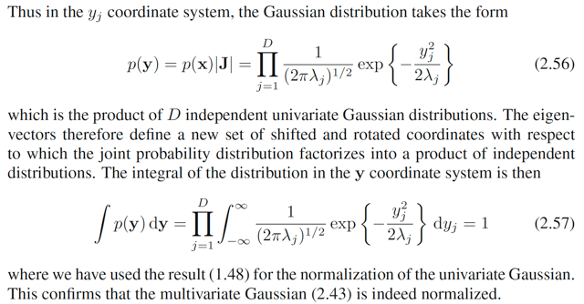
By de-correlation, the multi variate distribution can be the product of independent univariate distributions.
Pattern Recognition and Machine Learning (Christopher Bishop) - 2.3 The Gaussian Distribution

Related Resources
