Is my logistic regression model correct?

Question

I have a factorial design 2*2 (A and B). Both variables with two responses high (coded as 1) and low (coded as 0) and I have a response variable $y$, my logistic model include interaction between A and B in R, I coded logit<-glm(y~ A + B + A:B, data = df, family = "binomial").

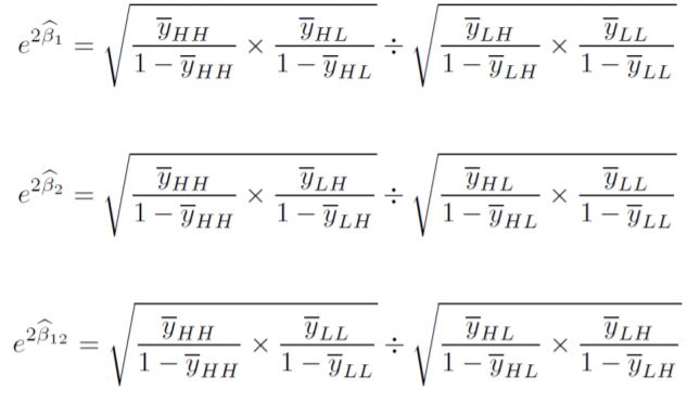
I verified the data and everything is good. I even ensured the my variables are coded as factors, in the exercise I'm working on I demonstrated that (check the image)

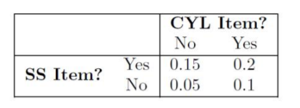
The $y$ in the picture are the average response. The table used to calculate the coefficient is :

The coefficient I found using the formulas in the picture are not equal to the coefficient in the output of R (see image)

I don't understand where the problem is. I hope someone can explain to me the error I made.

Thank you.

Answer 1

The coefficients you see in the glm() output are those in the following formulation:

$\log(\frac{p}{1-p}) = \beta_0 + \beta_1x_1 + \beta_2x_2 + \beta_3x_1x_2$

These coefficients do not correspond to probabilities of class membership: they are partial derivatives of the log-odds (logit) of your response variable being 1 with respect to your regressors. You can rearrange the above to give:

$\hat{p} = \frac{\exp(\beta_0 + \beta_1x_1 + \beta_2x_2 + \beta_3x_1x_2)}{1 + \exp(\beta_0 + \beta_1x_1 + \beta_2x_2 + \beta_3x_1x_2)}$

To see that this works, let's plug in CYL1=1 and SS1=0. Don't forget the intercept.

$\hat{p} = \frac{\exp(-2.9 + 0.75*1 + 1.2*0 - .39*1*0)}{1 + \exp(-2.9 + 0.75*1 + 1.2*0 - .39*1*0)} = \frac{\exp(-2.9 + 0.75)}{1 + \exp(-2.9 + 0.75)} = 0.1$

This gives us the bottom-right value in your table. Doing this for all four possibilities should give you the values in the table.

If you want to use predict() to predict the probabilities of future data, supply the type = "response" argument in order to have the output in this probability form. Otherwise, you will be given predicted log odds values.

Answer 2

You are calculating a function of exponentiated coefficients by plugging in probabilities from the model, R is reporting the index function coefficients that give you those probabilities. For example, the inverse logit of $-2.9444$ is $0.05$. You can use this to calculate the various $\bar y$s (or you can just calculate $y$ in each cell). The intercept corresponds to the low-low condition, so this matches the $\bar y_{LL}$ cell. I can reconstruct the exponentiated coefficients from ratios of the odds-ratios like this:

. scalar yll = invlogit(-2.9444)

. scalar yhl = invlogit(-2.9444 + 0.7472)

. scalar ylh = invlogit(-2.9444 + 1.2098)

. scalar yhh = invlogit(-2.9444 + 0.7472 + 1.2098 - 0.3989)

. 
. display "exp(alpha) = " exp(-2.9444)
exp(alpha) = .05263363

. display "exp(alpha) = " yll/(1-yll)
exp(alpha) = .05263363

. 
. display "exp(beta_1) = " exp(0.7472)
exp(beta_1) = 2.1110807

. display "exp(beta_1) = " ( yhl/(1-yhl) ) / ( yll/(1-yll) )
exp(beta_1) = 2.1110807

. 
. display "exp(beta_2) = " exp(1.2098)
exp(beta_2) = 3.352814

. display "exp(beta_2) = " ( ylh/(1-ylh) ) / ( yll/(1-yll) )
exp(beta_2) = 3.352814

. 
. display "exp(beta_12) = " exp(-0.3989)
exp(beta_12) = .6710578

. display "exp(beta_12) = " ((yhh/(1-yhh))/(yll/(1-yll)))/(( yhl/(1-yhl) ) / ( yll/(1-yll) )*( ylh/(1-ylh) ) / ( yll/(1-yll) ))
exp(beta_12) = .6710578

This is using the fact that since your model is

$$\ln \frac{p(d_1,d_2)}{1-p(d_1,d_2)} = \alpha + \beta_1 \cdot d_1 + \beta_2 \cdot d_2 + \beta_{12} \cdot d_{12},$$

when you take the exponent of both sides, you get $$ \begin{align} \frac{p(d_1,d_2)}{1-p(d_1,d_2)} &= \exp( \alpha + \beta_1 \cdot d_1 + \beta_2 \cdot d_2 + \beta_{12} \cdot d_{12} ) \\ & =\exp(\alpha) \cdot \exp(\beta_1 \cdot d_1) \cdot \exp( \beta_2 \cdot d_2) \cdot \exp(\beta_{12} \cdot d_{12} ). \end{align}$$

For example,

$$ \begin{align} \frac{p(d_1=0,d_2=0)}{1-p(d_1=0,d_2=0)} &= \exp(\alpha), \end{align}$$

since $\exp(\beta \cdot 0) = 1.$ Here $p(d_1=0,d_2=0) = \bar y_{LL}.$

Then we move on to $\exp{\beta_1}$. From above, we know that

$$ \begin{align} \frac{p(d_1=1,d_2=0)}{1-p(d_1=1,d_2=0)} =\exp(\alpha) \cdot \exp(\beta_1).\end{align}$$

We already know what the first term on the right-hand side is from the previous step, and we can calculate the left-hand side, so we just need to divide through by $\exp(\alpha)$ to get $\exp(\beta_1)$.

Similarly, $$\exp(\beta_{12}) = \frac{ \frac{p(d_1=1,d_2=1)}{1-p(d_1=1,d_2=1)}}{\exp(\alpha) \cdot \exp(\beta_1) \cdot \exp( \beta_2))},$$

which is the odds ratio for $y_{HH}$ over the product of the other three odds ratios. You can definitely rearrange terms a bit here to simplify since all the $\frac{\bar y_{LL}}{1-\bar y_{LL}}$ terms should cancel out.

However, I don't know where the square roots or the twos in your formula are coming from.