Coordinates from noisy distance matrix?

Question

I have a black box in which I know there is a 1D line and points along this line, and as output from this box I can get out a distance matrix for the points, but I know there is noise in the estimate for a given pair of points' distance. The diagonal of the output distance matrix is always zero and the upper half is simply *-1 of the lower half (i.e. sign of the distance is available). So, for example, here's some points and a custom noisy distance calculator that yields the kind of distance matrix I get as output:

set.seed(1)
x = c(1,3,4)
noisy_dist = function(x){
    out = matrix(0,nrow=length(x),ncol=length(x))
    for(i in 1:(length(x)-1)){
        for(j in (i+1):length(x)){
            out[i,j] = x[i] - x[j] + rnorm(1,0,.1)
            out[j,i] = -out[i,j]
        }
    }
    return(out)
}
D = noisy_dist(x)
print(D)
#          [,1]       [,2]       [,3]
# [1,] 0.000000 -2.0810097 -3.2430909
# [2,] 2.081010  0.0000000 -0.8850024
# [3,] 3.243091  0.8850024  0.0000000

So if I can only observe D, what would be appropriate approaches to using the observed information in this noisy distance matrix to estimate the latent location of the points?

Answer 1

Letting the coordinates of $p$ points be $\beta_i,$ $i=1,\ldots, p,$ the signed distances with noise are $$y_{ij} = \beta_i - \beta_j + \epsilon_{ij}=\mathbf{x}_{ij}\beta + \epsilon_{ij}$$ with iid Normal errors $\epsilon_{ij}$ and model matrix $x_{ij,k} = \delta_{ik}-\delta_{jk}.$

Not all $p$ coefficients are identifiable, however, because the distances don't determine the location. But if we arbitrarily fix one of the coefficients, say $\beta_1=0,$ we can estimate all the other locations relative to this one.

This is an Ordinary Least Squares (OLS) problem and so can be solved with the usual OLS machinery.

---

To illustrate, I generated four random points at locations

1.9 11.6  5.6  9.3

The model matrix $X = (x_{ij, k})$ (with its first column, for $\beta_1,$ omitted) is

        Point
Interval  2  3 4
     1-2  1  . .
     1-3  .  1 .
     1-4  .  . 1
     2-3 -1  1 .
     2-4 -1  . 1
     3-4  . -1 1

For instance, the first row in this matrix says the distance between points 1 and 2 equals $(1,0,0) (\beta_2,\beta_3,\beta_4)^\prime = \beta_2 = \beta_2-\beta_1$ (because, implicitly, $\beta_1=0$). The last row says the distance between points 3 and 4 is $-\beta_3 + \beta_4.$

The least squares estimates, compared to the locations, are good:

                2   3   4
True location 9.8 3.8 7.5
Estimate      9.8 3.1 7.8

(Notice that "true location" is relative to the first point at 1.9.)

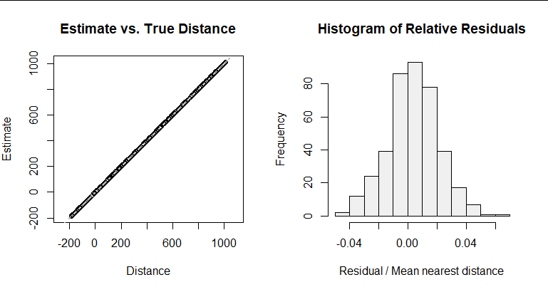
As another illustration, I created 400 random points (at typical inter-point distances of $3$) and measured their $400(399)/2=159\,600$ distances with Gaussian noise of unit standard deviation (which is a fairly large fraction of these distances, making this a stringent test). Rather than print out the results, it's better to graph the $399$ coefficient estimates!

You can see it works very well. The reason is that we have $399$ measurements associated with each point, so the imprecision in each estimate should be about $1/\sqrt{399}\approx 0.05,$ or about $1.7\%$ of the average nearest-neighbor distance. The imprecision is about twice that because these measurements are not independent.

The software fit this model (of $159\,600$ observations and $399$ variables) in a couple of seconds. I used a sparse matrix for $X$ to save RAM.

---

This is the complete R code for generating the examples and figures. (Change n <- 4 to n <- 400 for the figures.) The estimates are stored in the vector b.

noisy_dist = function(x, sigma=1){
  out <- as.matrix(dist(x)) 
  eps <- matrix(0, nrow(out), ncol(out))
  i <- lower.tri(eps)
  eps[i] <- rnorm(sum(i), 0, sigma)
  (out + eps + t(eps)) * outer(x, x, function(i,j) sign(i-j)) # Signed distance
}
#
# Create a noisy distance matrix.
#
set.seed(17)
n <- 4
x <- runif(n, 0, 3*n)
names(x) <- seq_along(x)
if (length(x) <= 10) print(x, digits=2)

D = noisy_dist(x)
if (length(x) <= 10) print(D, digits=2)
#
# Create the model matrix associated with `D`.
#
library(Matrix)
X <- (function(ij) {
  f <- function(u) 
    sparseMatrix(i=seq_len(ncol(ij)), j=ij[u,], x=(-1)^u, dims=c(ncol(ij), max(ij))) 
  X <- f(1) + f(2)
  dimnames(X) <- list(Interval=paste(ij[1,], ij[2,], sep="-"), Point=seq_len(max(ij)))
  X
})(combn(seq_len(nrow(D)), 2))
if (length(x) <= 10) print(X[, -1])
#
# Estimate the coefficients.
#
library(MatrixModels)
b <- MatrixModels:::lm.fit.sparse(X[, -1], D[lower.tri(D)])
if (length(b) < 10) round(rbind(`True location`=x[-1] - x[1], Estimate=b), 1)
#
# Display some diagnostic plots.
#
par(mfrow=c(1,2))
plot(x[-1] - x[1], b, asp=1,
     xlab="Distance", ylab="Estimate",
     main="Estimate vs. True Distance")
abline(c(0,1), lty=3, lwd=2, col="Gray")

sigma <- diff(range(x)) / (length(x) - 1)
hist((b - (x[-1] - x[1])) / sigma,  col="#f0f0f0",
     main="Histogram of Relative Residuals",
     xlab="Residual / Mean nearest distance")
par(mfrow=c(1,1))