For logistic models for inference, it's important to first underscore that there is no error here. The warning in R is correctly informing you that the maximum likelihood estimator lies on the boundary of the parameter space. The odds ratio of $\infty$ is strongly suggestive of an association. The only issue is that two common methods of producing tests: the Wald test and the Likelihood ratio test require an evaluation of the information under the alternative hypothesis.
With data generated along the lines of
x <- seq(-3, 3, by=0.1)
y <- x > 0
summary(glm(y ~ x, family=binomial))
The warning is made:
Warning messages:
1: glm.fit: algorithm did not converge
2: glm.fit: fitted probabilities numerically 0 or 1 occurred
which very obviously reflects the dependence that is built into these data.
In R the Wald test is found with summary.glm or with waldtest in the lmtest package. The likelihood ratio test is performed with anova or with lrtest in the lmtest package. In both cases, the information matrix is infinitely valued, and no inference is available. Rather, R does produce output, but you cannot trust it. The inference that R typically produces in these cases has p-values very close to one. This is because the loss of precision in the OR is orders of magnitude smaller that the loss of precision in the variance-covariance matrix.
Some solutions outlined here:
Use a one-step estimator,
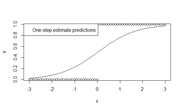
There is a lot of theory supporting the low bias, efficiency, and generalizability of one step estimators. It is easy to specify a one-step estimator in R and the results are typically very favorable for prediction and inference. And this model will never diverge, because the iterator (Newton-Raphson) simply does not have the chance to do so!
fit.1s <- glm(y ~ x, family=binomial, control=glm.control(maxit=1))
summary(fit.1s)
Gives:
Coefficients:
            Estimate Std. Error z value Pr(>|z|)
(Intercept) -0.03987    0.29569  -0.135    0.893
x            1.19604    0.16794   7.122 1.07e-12 ***
---
Signif. codes:  0 ‘***’ 0.001 ‘**’ 0.01 ‘*’ 0.05 ‘.’ 0.1 ‘ ’ 1
So you can see the predictions reflect the direction of trend. And the inference is highly suggestive of the trends which we believe to be true.

perform a score test,
The Score (or Rao) statistic differs from the the likelihood ratio and wald statistics. It does not require an evaluation of the variance under the alternative hypothesis. We fit the model under the null:
mm <- model.matrix( ~ x)
fit0 <- glm(y ~ 1, family=binomial)
pred0 <- predict(fit0, type='response')
inf.null <- t(mm) %*% diag(binomial()$variance(mu=pred0)) %*% mm
sc.null <- t(mm) %*% c(y - pred0)
score.stat <- t(sc.null) %*% solve(inf.null) %*% sc.null ## compare to chisq
pchisq(score.stat, 1, lower.tail=F)
Gives as a measure of association very strong statistical significance. Note by the way that the one step estimator produces a $\chi^2$ test statistic of 50.7 and the score test here produces a test statistic pf 45.75
> pchisq(scstat, df=1, lower.tail=F)
             [,1]
[1,] 1.343494e-11
In both cases you have inference for an OR of infinity.
, and use median unbiased estimates for a confidence interval.
You can produce a median unbiased, non-singular 95% CI for the infinite odds ratio by using median unbiased estimation. The package epitools in R can do this. And I give an example of implementing this estimator here: Confidence interval for Bernoulli sampling


