combining a random variable and its inverse

Question

I am measuring two scientific entities, X and Y using empiric measurements. Each has its own mean and sample variance based on Nx and Ny sample measurements. I know from the underlying science that X is 1/Y (e.g. one variable is the inverse of the other). Because the sampling is empiric I don't get a result which is exactly inverse. I want to make the best estimate of the ratio between them. e.g. let X have a mean of 4 based on 30 measurements with a stdev of 3. let Y have a mean of 0.4 based on 12 measurements with stdev of 0.5

so combining the two I should have something like X=3 and Y=1/3 But maybe it should be X=3.5 and Y=1/3.5 etc..

How do I go about finding the best ratio?

Answer 1

It sounds like you have a dataset consisting of measurements $(x_i, i=1,2,\ldots,n)$ and $(y_j, j=1,2,\ldots,m)$ (with $n=30, m=12$). Let us posit that

1. All the measurements can be considered independent random variables.

2. There is a fixed number ("parameter") $\mu$ for which all $x_i-\mu$ have a common distribution $F$ (whose expectation is $0$, reflecting a lack of bias in those measurements) and all the $y_j - 1/\mu$ have a common distribution $G$ (also with $0$ expected value).

One way to make some progress is to study the error distributions $F$ and $G$. To illustrate how this information can be used, let us consider a widely applicable model in which the distributions have identical shapes but unknown amounts of dispersion (which we will measure with the variance). Let the variance of $F$ be $\sigma^2$ and the variance of $G$ be $\tau^2$. Often these distributions will be approximately Normal, for instance (although many other forms of error can be modeled).

The independence assumptions imply the likelihood of the observations, $L$, is the product of their individual probability densities. Let $\phi$ be the density for a unit variance. When we assume Normally-distributed variation, for instance,

$$\phi(z) = \frac{1}{\sqrt{2\pi}} \exp({-z^2/2}).$$

Then $\phi_\sigma(x) = \phi(x/\sigma)/\sigma$ is the density of $F$ and $\phi_\tau(y)=\phi(y/\tau)/\tau$ is the density of $G$. Accordingly,

$$L(\mu, \sigma, \tau; (x_i), (y_j)) = \prod_{i=1}^n \phi_\sigma(x_i-\mu) \prod_{j=1}^m \phi_\tau(y_j-1/\mu).$$

We may estimate $\mu$ using the method of Maximum Likelihood: find values of $\mu,\sigma,\tau$ that make this likelihood as large as possible. To simplify the products, and to conform with a convention that optimization problems are usually cast as minimization problems, let us minimize the negative log likelihood

$$\eqalign{ \Lambda(\mu,\sigma,\tau) &= -\log(L(\cdots)) \\ &= -\sum_{i=1}^n \left(\log \phi\left(\frac{x_i-\mu}{\sigma}\right) - \log \sigma \right) - \sum_{j=1}^m \left(\log \phi\left(\frac{y_j-1/\mu}{\tau}\right) - \log \tau \right) \\ &=-n\log\sigma - m\log\tau - \sum_{i=1}^n \log \phi\left(\frac{x_i-\mu}{\sigma}\right) - \sum_{j=1}^m\log \phi\left(\frac{y_j-1/\mu}{\tau}\right). }$$

To continue the illustration, assume from now on that the error distributions are Normal. We easily find that the minimum must occur when $\sigma^2$ is the variance of the $(x_i)$ and $\tau$ is the variance of the $(y_j)$:

$$\hat\sigma^2 = \frac{1}{n} \sum_{i=1}^n (x_i - \bar x)^2; \quad \bar x = \frac{1}{n}\sum_{i=1}^n x_i; \\ \hat\tau^2= \frac{1}{m} \sum_{i=1}^m (y_i - \bar y)^2; \quad \bar y = \frac{1}{m}\sum_{j=1}^m y_j.$$

It remains to find $\hat\mu$ for which $\Lambda(\hat\mu,\hat\sigma,\hat\tau)$ is minimum. This value could be any real number--there are no boundary values to check. Since $\Lambda$ is a differentiable function of its first argument, the minimum must occur at a zero of its derivative:

$$0 = \frac{\partial}{\partial \mu}\Lambda(\mu,\cdots) = \frac{1}{ \hat\sigma }\sum_{i=1}^n \frac{\phi^\prime\left(\frac{x_i-\mu}{\hat\sigma}\right)}{ \phi\left(\frac{x_i-\mu}{\hat\sigma}\right) } - \frac{1}{\mu^2 \hat\tau}\sum_{j=1}^m \frac{\phi^\prime\left(\frac{y_j-1/\mu}{\hat\tau}\right)}{ \phi\left(\frac{y_j-1/\mu}{\hat\tau}\right) }. $$

Normal distributions are often chosen in models precisely because the function $\phi^\prime(z)/\phi(z) = -z$ is linear, making such equations easy to solve. In this case the presence of $1/\mu$ complicates things a bit:

$$\frac{n}{\hat \sigma^2}\left(\bar x - \mu\right) = \frac{1}{\hat\sigma}\sum_{i=1}^n \frac{x_i - \mu}{\hat\sigma} = \frac{1}{\mu^2\hat\tau}\sum_{j=1}^m\frac{y_j - 1/\mu}{\hat\tau} = \frac{m}{\mu^2\hat\tau^2}\left(\bar y - 1/\mu\right).$$

The equation in $\mu$, whose solutions must include the estimate $\hat\mu$, is of fourth degree, rather than linear. Nevertheless it can be solved numerically and typically will produce a global minimum somewhere near $\bar x$ or $1/\bar y$, provided there are enough data and their variances are not too large. (The presence of negative values is not a good sign!)

(Alternatively, we might hope that the variance of $y$ decreases with $\mu$, as is often the case in measuring positive quantities. In that case we might discover that the $y_j$ are perhaps better modeled using distributions whose variances are $\tau^2/\mu^2$ (for example). This would turn the preceding equation back into one which is linear in $\mu$, making it straightforward to solve. This possibility suggests there is value in studying how the precision of the measurement process producing the $y_j$ might vary with $\mu$. The $x_i$ measurement process deserves a comparable study.)

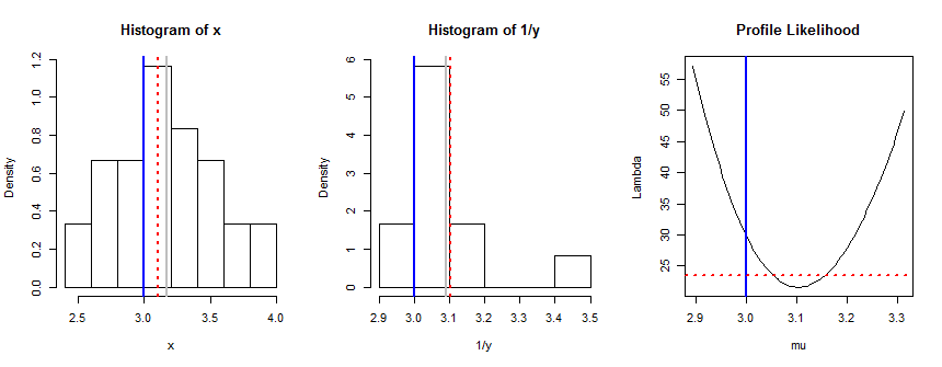
Simulations suggest that with the conditions described in the question ($\bar x$ near $3$, $n=30$, $m=12$, and some negative values in the $y$ data), using the $y$ data actually does not improve the precision of the estimates. The estimates are improved when the aggregate $y$ measurements are relatively more precise than the aggregate $x$ measurements; that is, when $m\tau^2 \mu^2 \gg n\sigma^2 / \mu^2$ ($\tau \ll \frac{m}{n}\sigma/\mu^2$), assuming $\mu \gt 1$. Here is an example of that good situation, and indeed $\hat\mu$ is closer to $\mu$ than $\bar x$ is:

The vertical solid blue lines are the true mean $\mu=3$. The vertical solid gray lines show the means $\bar x$ and $1/\bar y$. The vertical dashed red lines show the ML estimate $\hat\mu$. The horizontal dashed red line in the Profile Likelihood plot shows an upper $95\%$ confidence limit for $\Lambda$: values of $\mu$ for which the graph of $\Lambda$ lie below this limit form a two-sided $95\%$ confidence interval for $\mu$. In this example that interval does not include the true value of $\mu$. However--as you can check--re-running this example with different randomly-generated data will produce intervals that include the true value $95\%$ of the time.

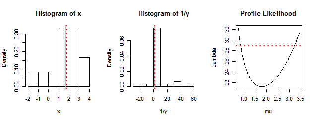
FWIW, applying this procedure to the data (as given in a comment to another answer, interpreting the 12 values of "first var" to be $x$ and the 30 values of "second var" to be $y$) yields $\hat\mu = 1.79$, with a $95\%$ confidence interval approximately $[1.2,2.5]$. The data reflect a large amount of measurement error: $\hat\sigma=1.85$ and $\hat\tau=1.40$. Here is a summary of the data and the fit:

NB The dashed horizontal red line in the right-hand plot is too high: it should be located around $23.5$.

Here is the R code to compute $\hat\mu, \hat\sigma, \hat\tau$, and to conduct such simulations.

#
# Negative log (partial) likelihood.
#
lambda <- function(mu, sigma2, tau2, x, y) {
  (sum((x - mu)^2)/sigma2 + sum((y - 1/mu)^2)/tau2)/2
}
#
# Maximum likelihood estimation.
#
mle <- function(x, y) {
  sigma.hat <- mean((x-mean(x))^2)
  tau.hat <- mean((y-mean(y))^2)
  fit <- optimize(lambda, c(min(1/max(y), min(x)), max(x, 1/min(y))),
                  sigma2=sigma.hat, tau2=tau.hat, x=x, y=y)
  list(mu.hat=fit$minimum, sigma.hat=sigma.hat, tau.hat=tau.hat, 
       Lambda=fit$objective)
}
#
# Create sample data.
#
set.seed(17)
n <- 30; m <- 12
mu <- 3
sigma <- 1/2
tau <- 0.5 * (m/n) * sigma / mu^2
x <- rnorm(n, mu, sigma)
y <- rnorm(m, 1/mu, tau)
#
# Find the solution.
#
fit <- mle(x, y)
#
# Plot the data and profile log likelihood
#
se <- sd(x) / sqrt(n)
i <- seq(fit$mu.hat-3*se, fit$mu.hat+3*se, length.out=101)
z <- sapply(i, function(j) lambda(j, fit$sigma.hat, fit$tau.hat, x, y))
markup <- function(z) {
  abline(v = mu, col="Blue", lwd=2)
  if(!missing(z)) abline(v = z, col="Gray", lwd=2)
  abline(v = fit$mu.hat, lwd=2, col="Red", lty=3) #$
}
par(mfrow=c(1,3))
hist(x, freq=FALSE); markup(mean(x))
hist(1/y, freq=FALSE); markup(1/mean(y))
plot(i, z, type="l", xlab="mu", ylab="Lambda", main="Profile Likelihood")
abline(v = mu, col="Blue", lwd=2)
abline(h = fit$Lambda + qchisq(0.95, 1)/2, lty=3, lwd=2, col="Red")

Answer 2

I want to complete whuber answer (very nice as always) with some distribution free considerations.

I denote $E(Z) = m$ and $\text{Var}(Z) = \sigma^2$ by $Z\sim (m, \sigma^2)$.

First, a small lemma (using Delta method) : if $Z \sim \left({1\over \mu}, \sigma^2\right)$, then approximately ${1\over Z} \sim \left( \mu + \mu^3 \sigma^2, \mu^2\sigma^2\right)$. This comes readily from the first and second order approximations $$\begin{aligned} {1\over Y} = {1\over {1\over \mu} + Y - {1\over \mu}} &\simeq \mu - \mu^2 \left(Y-{1\over\mu}\right)\\ &\simeq \mu - \mu^2 \left(Y-{1\over\mu}\right)+\mu^3\left(Y-{1\over\mu}\right)^2. \end{aligned}$$ Note that you need to assume that the support of the law is in $\mathbb R^{>0}$ or in $\mathbb R^{<0}$ for this to make sense.

Now assume $Y_1, \dots, Y_m$ are independent $~\sim\left({1\over \mu},\sigma^2\right)$. There are two natural ways to find an estimate of $\mu$, and from the above lemma we can find approximations of their expected value and variance:

$$\begin{aligned} {1\over m} \left( {1\over Y_1} + \cdots + {1\over Y_m} \right) &\sim \left( \mu + \mu^3 \sigma^2, {1\over m}\mu^2\sigma^2 \right) \\ {m \over Y_1 + \cdots + Y_m} &\sim \left( \mu + {1\over m} \mu^3 \sigma^2, {1\over m}\mu^2\sigma^2 \right) \end{aligned}$$

The second one a bias in $1 \over m$, where as the first has constant bias. This is somehow intuitive, but I think this was worth mentioning.

Answer 3

Say you have two sets of data: $x_i$ and $y_j$. We know that $\frac{1}{y_j}=x_j$ from theory or the previous research. I think the best estimate of the average $\bar x$ is the following: $$\bar x=\frac{\sum_{n_x}x_i+\sum_{n_y}\frac{1}{y_j}}{n_x+n_y}$$

Let's see if it's biased: $$E[\bar x - \mu]=\frac{\sum_{n_x}(E[x_i]-\mu)+\sum_{n_y}(E[\frac{1}{y_j}]-\mu)}{n_x+n_y}=0$$

This is because $$E[\frac{1}{y_j}]=E[x_j]=\mu$$ Note, that $E[y]\ne\frac{1}{\mu}$

If you want to compare the ratios, then proceed in a similar fashion:

$$\mu_x=\frac{\sum_{i=1}^{n_x}x_i}{n_x}$$ and $$\mu_y=\frac{\sum_{j=1}^{n_y}\frac{1}{y_j}}{n_x}$$

the same goes for standard deviations and the usual t-test ANOVA: use $\frac{1}{y_j}$ wherever you use used $x_i$. The key here is not to work on aggregates, such as $E[y_j]$, because they're not convertible easily into $\frac{1}{E[x]}$ due to Jensen inequality.

UPDATE Here's analogy from physics. Let's say you're measuring the resistance. You have Ohm-meter, which measures it directly and shows 10 Ohm.

Now, you measure it with a Ampere-meter by connecting the resistor to the DC power supply which produces 10 Volt. Ohm's Law: $R=\frac{V}{I}$. You read two measurements: 1.1 A and 1.2 A.

I'm suggesting you compare 10 $\Omega$ with $\frac{\frac{10}{1.1}+\frac{10}{1.2}}{2}=8.7 \Omega$

UPDATE2: Based on OP's comments, it seems the model is as follows: $$x_i=z_i+e_i$$ $$y_j=\frac{1}{z_j}+u_j$$ Here, $z$ is what we want to measure, while $x$ and $y$ are what we actually measure, and $e,u$ are errors, which are quite large.

If you go with combining $E[x]$ and $\frac{1}{E[y]}$, then you'll have to deal with the bias $\frac{1}{E[y]}-E[z]$.

I think in this case it is important to understand the errors, especially $u_j$. If we knew something about the distribution, we could correct for bias.