This is a difficult problem. I thought first about using (some approximation of) the moment generating function of the lognormal distribution. That doesn't work, as I will explain. But first some notation:
Let $\phi$ be the standard normal density and $\Phi$ the corresponding cumulative distribution function. We will only analyze the case lognormal distribution $lnN(0,1)$, which has density function
$$
f(x)=\frac1{\sqrt{2\pi}x} e^{-\frac12 (\ln x)^2}
$$
and cumulative distribution function
$$
F(x) =\Phi(\ln x)
$$
Suppose $X$ and $Y$ are independent random variables with the above lognormal distribution. We are interested in the distribution of $D=X-Y$, which is a symmetric distribution with mean zero. Let $M(t) = \DeclareMathOperator{\E}{E} \E e^{tX} $ be the moment generating function of $X$. It is defined only for $t\in (-\infty,0]$, so not defined in an open interval containing zero. The moment generating function for $D$ is $M_D(t)=\E e^{t(X-Y)}= \E e^{tX} \E e^{-tY}= M(t)M(-t)$. So, the moment generating function for $D$ is only defined for $t=0$, so not very useful.
That means we will need some more direct approach for finding approximations for the distribution of $D$. Suppose $t\ge 0$, calculate
$$
\begin{align}
P(D \le t) &= P(X-Y\le t) \\
&= \int_0^\infty P(X-y\le t | Y=y) f(y) \; dy \\
&= \int_0^\infty P(X\le t+y) f(y) \; dy \\
&= \int_0^\infty F(t+y) f(y) \; dy
\end{align}
$$ (and the case $t<0$ is solved by symmetry, we get $P(D\le t)=1-P(D\le |t|)$).
This expression can be used for numerical integration or as a basis for simulation. First a test:
 integrate(function(y) plnorm(y)*dlnorm(y), lower=0,  upper=+Inf)
  0.5 with absolute error < 2.3e-06
which is clearly correct. Let us wrap this up inside a function:
pDIFF  <-  function(t) {
    d  <-  t
    for (tt in seq(along=t)) {
        if (t[tt] >= 0.0) d[tt] <- integrate(function(y) plnorm(y+t[tt])*dlnorm(y),
                                         lower=0.0,  upper=+Inf)$value else
                          d[tt] <- 1-integrate(function(y) plnorm(y+abs(t[tt]))*dlnorm(y),
                                         lower=0.0, upper=+Inf)$value
    }
    return(d)
}

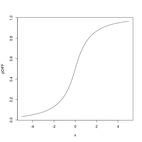
> plot(pDIFF,  from=-5,  to=5)
which gives:

Then we can find the density function by differentiating under the integral sign, obtaining
dDIFF  <-  function(t) {
       d  <- t; t<- abs(t)
       for (tt in seq(along=t)) {
           d[tt]  <-  integrate(function(y) dlnorm(y+t[tt])*dlnorm(y),
                                lower=0.0,  upper=+Inf)$value
       }
       return(d)
}
which we can test:
> integrate(dDIFF,  lower=-Inf,  upper=+Inf)
0.9999999 with absolute error < 1.3e-05
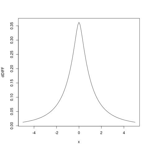
And plotting the density we get:
plot(dDIFF, from=-5, to=5)

I did also try to get some analytic approximation, but so far didn't succeed, it is not an easy problem. But numerical integration as above, programmed in R is very fast on modern hardware, so is a good alternative which probably should be used much more.


