50
$\begingroup$

I am wondering what we can say, if anything, about the population mean, $\mu$ when all I have is one measurement, $y_1$ (sample size of 1). Obviously, we'd love to have more measurements, but we can't get them.

It seems to me that since the sample mean, $\bar{y}$, is trivially equal to $y_1$, then $E[\bar{y}]=E[y_1]=\mu$. However, with a sample size of 1, the sample variance is undefined, and thus our confidence in using $\bar{y}$ as an estimator of $\mu$ is also undefined, correct? Would there be any way to constrain our estimate of $\mu$ at all?

$\endgroup$
4
  • $\begingroup$ Yes, a confidence interval on $\mu$ can be constructed under certain assumptions. If no one posts it, I will track it down. $\endgroup$
    – soakley
    Commented Jun 18, 2015 at 15:43
  • 6
    $\begingroup$ See stats.stackexchange.com/questions/1807 for another version of the same question (the average of a sample is available, but not its sample size, so effectively the average is a single observation from the unknown sampling distribution) and stats.stackexchange.com/questions/20300 for a related discussion. $\endgroup$
    – whuber
    Commented Jun 18, 2015 at 16:49
  • $\begingroup$ a recent article discussing optimality of these estimators in the normal case: tandfonline.com/doi/full/10.1080/00031305.2017.1360796 $\endgroup$
    – user795305
    Commented Sep 19, 2017 at 12:59
  • $\begingroup$ See Edelman, D (1990) 'A confidence interval for the center of an unknown unimodal distribution based on a sample size one' The American Statistician, Vol 44, no 4. Article covers the Normal and Nonparametric cases. $\endgroup$ Commented Oct 16, 2019 at 18:16

5 Answers 5

9
$\begingroup$

Here is a brand-new article on this question for the Poisson case, taking a nice pedagogical approach:

Andersson. Per Gösta (2015). A Classroom Approach to the Construction of an Approximate Confidence Interval of a Poisson Mean Using One Observation. The American Statistician, 69(3), 160-164, DOI: 10.1080/00031305.2015.1056830.

$\endgroup$
5
  • $\begingroup$ ...unfortunately behind a paywall. $\endgroup$
    – Tim
    Commented Sep 2, 2015 at 8:35
  • 1
    $\begingroup$ @Tim: that is so. Then again, an ASA membership is not terribly expensive, and you get access to The American Statistician, JASA and quite a few other journals at a very reasonable price, which I personally very happily pay out of my own pocket. I really think you get your money's worth here. YMMV, of course. $\endgroup$ Commented Sep 2, 2015 at 8:39
  • 5
    $\begingroup$ +1 but the Poisson case is radically different from the normal case because the variance has to equal the mean. The Poisson result is pretty straightforward whereas the $x\pm 9.68 |x|$ result for the normal case is counter-intuitive and mysterious. $\endgroup$
    – amoeba
    Commented Feb 5, 2016 at 12:50
  • $\begingroup$ @amoeba: quite correct, but the OP did not specify any restrictions on the distribution. $\endgroup$ Commented Feb 5, 2016 at 13:36
  • 1
    $\begingroup$ This is so brief that it would better serve as a comment. But since it is the accepted answer, you probably will not wish to convert it to a comment. Could you then perhaps summarize the main points of the article? $\endgroup$ Commented Oct 16, 2019 at 19:40
42
$\begingroup$

If the population is known to be normal, a 95% confidence interval based on a single observation $x$ is given by $$x \pm 9.68 \left| x \right| $$

This is discussed in the article "An Effective Confidence Interval for the Mean With Samples of Size One and Two," by Wall, Boen, and Tweedie, The American Statistician, May 2001, Vol. 55, No.2. (pdf)

$\endgroup$
6
  • 5
    $\begingroup$ I hate to sound stupid but.... surely not. This depends on units and doesn't behave properly at all (by properly I mean scalar multiplication....) $\endgroup$
    – Alec Teal
    Commented Jun 19, 2015 at 5:48
  • 9
    $\begingroup$ @Alec Just because a procedure depends on units of measurement (that is, it is not invariant) does not mean it is automatically invalid or even bad. This one is valid: read the article and do the math. Many will grant that it is a little disturbing, though. Even more surprisingly, you don't even have to assume the underlying distribution is Normal: a similar result holds for any unimodal distribution (but 9.68 has to be increased to about 19 or so): see the links I provided in a comment to this question. $\endgroup$
    – whuber
    Commented Jun 19, 2015 at 13:29
  • 4
    $\begingroup$ A later issue of the journal had three letters to the editor, one of which brought up Alec Teal's point about the units. The reply from Wall says this: "The confidence interval is not equivariant (i.e., its coverage probability depends on the ratio of ${{\left| \mu \right| } \over {\sigma}}$...)" Later she says "The confidence interval is not based on a pivotal quantity..." It's an unusual approach and result, no doubt! $\endgroup$
    – soakley
    Commented Jun 19, 2015 at 13:35
  • 6
    $\begingroup$ Just to save y'all a bit of work: the letters to the editor & reply @soakley notes appeared in The American Statistician, vol. 56, no. 1 (2002). $\endgroup$ Commented Jun 19, 2015 at 18:54
  • 3
    $\begingroup$ This seems to give confidence intervals covering the mean with probability about $95\%$ when $\sigma \approx | \mu | \gt 0$ but with much higher probabilities otherwise. If $\mu = 0$ then clearly the probability is $100\%$ as the confidence intervals always contain $0$. $\endgroup$
    – Henry
    Commented Jun 19, 2015 at 22:05
30
$\begingroup$

Sure there is. Use a Bayesian paradigm. Chances are you have at least some idea of what $\mu$ could possibly be - for instance, that it physically cannot be negative, or that it obviously cannot be larger than 100 (maybe you are measuring the height of your local high school football team members in feet). Put a prior on that, update it with your lone observation, and you have a wonderful posterior.

$\endgroup$
7
  • 20
    $\begingroup$ (+1) One observation will be overwhelmed by the prior, so it would seem that what you get out of the posterior will not be much more than what you put into the prior. $\endgroup$
    – whuber
    Commented Jun 18, 2015 at 16:51
  • $\begingroup$ What if we combined such a prior with the kind of likelihood implied by that wretched $x \pm 9.68 \left|x\right|$? $\endgroup$ Commented Jun 19, 2015 at 20:25
  • $\begingroup$ @SimonKuang: one conceptual problem is that we can only use the $x\pm 9.68|x|$ interval after we have observed $x$, so this can't enter the prior. $\endgroup$ Commented Jun 20, 2015 at 5:21
  • $\begingroup$ @StephanKolassa No, this interval (and the associated distribution) forms the likelihood. Our prior is separate. $\endgroup$ Commented Jun 20, 2015 at 6:58
  • $\begingroup$ @SimonKuang: yes, you are right, my mistake. Unfortunately, I don't have the time to go through this at this time, but if you do this, please post what you find! $\endgroup$ Commented Jun 20, 2015 at 14:06
14
$\begingroup$

A small simulation exercise to illustrate whether the answer by @soakley works:

# Set the number of trials, M
M=10^6
# Set the true mean for each trial
mu=rep(0,M)
# Set the true standard deviation for each trial
sd=rep(1,M)
# Set counter to zero
count=0
for(i in 1:M){
 # Control the random number generation so that the experiment is replicable 
 set.seed(i)
 # Generate one draw of a normal random variable with a given mean and standard deviation
 x=rnorm(n=1,mean=mu[i],sd=sd[i])
 # Estimate the lower confidence bound for the population mean
 lower=x-9.68*abs(x)
 # Estimate the upper confidence bound for the population mean
 upper=x+9.68*abs(x)
 # If the true mean is within the confidence interval, count it in
 if( (lower<mu[i]) && (mu[i]<upper) ) count=count+1
}
# Obtain the percentage of cases when the true mean is within the confidence interval
count_pct=count/M
# Print the result
print(count_pct)
[1] 1

Out of one million random trials, the confidence interval includes the true mean one million times, that is, always. That should not happen in case the confidence interval was a 95% confidence interval.

So the formula does not seem to work... Or have I made a coding mistake?

Edit: the same empirical result holds when using $(\mu, \sigma)=(1000,1)$;
however, it is $0.950097 \approx 0.95$ for $(\mu, \sigma)=(1000,1000)$ -- thus pretty close to the 95% confidence interval.

$\endgroup$
18
  • 2
    $\begingroup$ Indeed, for $\mu$ not equal to 0, this is useful (and +1 for providing the code in the first place!). I just meant that for $\mu = 0$, it's a foregone conclusion that 0 will always be captured. $\endgroup$
    – Wolfgang
    Commented Jun 19, 2015 at 13:13
  • 3
    $\begingroup$ (@Wolfgang) This is not the way to test a confidence interval. The definition does not require that the $\alpha$-level CI covers the mean $1-\alpha$ of the time in every case: it requires only that (a) has at least that much coverage in every case and (b) it approximates that coverage in some cases. Thus, for your approach to be valid and convincing you would have to search a large number of possibilities. Try sim <- function(rho, n.iter=1e5, sigma=1, psi=9.68) { mu <- runif(n.iter, 0, sigma) * rho; x <- rnorm(n.iter, mu, sigma); mean(p <- abs(x - mu) <= psi * abs(x)) }; sim(1.75) $\endgroup$
    – whuber
    Commented Jun 19, 2015 at 13:25
  • 2
    $\begingroup$ I understand the point you are trying to make, but I strongly disagree with the statement that "this is not the way to test a confidence interval". In the definition/construction of a CI, the parameter is a fixed constant. In your simulation, $\mu$ keeps changing. For fixed $\mu$, if the method truly gives a 95% CI, then it should cover $\mu$ in 95% of the cases. It doesn't. Also, even with your construction, sim(0.1) yields a coverage very close to 1 (of course, now we are getting closer again to $\mu$ being fixed at 0). $\endgroup$
    – Wolfgang
    Commented Jun 19, 2015 at 13:37
  • 2
    $\begingroup$ @Wolfgang check the definition used by paper quoted, it is: $P(X - \zeta |X| \leq \mu \leq X + \zeta |X|) \geq 1 - \alpha $, i.e. the probability that $\mu$ is in the interval is at least 0.95. $\endgroup$
    – Tim
    Commented Jun 19, 2015 at 17:45
  • 3
    $\begingroup$ Again, $\mu$ is a constant. So, it's perfectly fine to simulate with $\mu = 0$. Of course, then coverage must be 1. The method provides a CI that has at least 95% coverage and the example shows (whether by simulation or via reasoning) that in some conditions, coverage could be as high as 100%. So, it's not a 95% CI. It's still a pretty clever method for drawing some kind of inference from so little information. $\endgroup$
    – Wolfgang
    Commented Jun 20, 2015 at 7:13
0
$\begingroup$

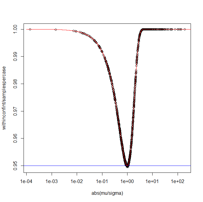
Here is a simulation to demonstrate that @soakley's confidence interval works for a normally distributed random variable.

  • It takes $10^4$ values of $\mu$ in $[-10,10]$ and of $\sigma$ in $[0,10]$ and
  • for each of those pairs, it generates $10^6$ single observations $x$ and
  • sees what proportion of the corresponding confidence intervals $[x- 9.68|x|, x+9.68|x|]$ cover $\mu$.
  • It then plots this proportion against $\frac{|\mu|}{\sigma}$ as small black circles to illustrate when this proportion is about $0.95$ (the blue line) and when it is much higher.
  • The red line shows the theoretical confidence for varying values of $\frac{|\mu|}{\sigma}$.

Using R:

set.seed(2023)
cases <- 10^3
samplespercase <- 10^6
mu <- runif(cases)*20-10
sigma <- runif(cases)*10
withinconfint <- numeric(cases)
for (i in 1:cases){
    sample <- rnorm(samplespercase, mean=mu[i], sd=sigma[i])
    withinconfint[i] <- sum(sample - 9.68*abs(sample) < mu[i] &
                            sample + 9.68*abs(sample) > mu[i])
    }
plot(abs(mu/sigma), withinconfint/samplespercase, log="x")
abline(h=0.95,col="blue")
curve(pnorm(x/(1-9.68),x,1) + 1 - pnorm(x/(1+9.68),x,1),
      from=10^-4, to=10^4, col="red", n=50001, log="x", add=TRUE)
enter image description here

Taking account of simulation noise, this suggests the claim and the corresponding expression for theoretical confidence of $\Phi\left(\frac{9.68}{(1-9.68)x}\right) + 1 - \Phi\left(\frac{-9.68}{(1+9.68)x}\right)$ are highly plausible. When $\frac{|\mu|}{\sigma} \approx 1$ the confidence is marginally above $0.95$, though at other times it is much more conservative and closer to $1$.

The chart seems to suggest the minimum confidence is when $\frac{|\mu|}{\sigma} = 1$; this is not quite correct and for $\alpha=1-0.95=0.05$ it is closer to $0.99$; for larger $\alpha < \frac12$ it would be at an even lower value of $\frac{|\mu|}{\sigma}$.

Meanwhile the $9.68$ is marginally higher than $\sqrt{\frac{2}{e\pi}} /\alpha \approx \frac{0.48394}{\alpha}$ and needs to be. For all $\alpha < \frac12$ we can use the slightly more conservative $\frac{0.5}{\alpha}$ and so a confidence interval of $\left[x-\frac1{2\alpha}|x|, x+\frac1{2\alpha}|x|\right]$ to have a probability of over $1-\alpha$ of covering the unknown mean, which in this example would have been $x\pm 10|x|$ which would have given confidence of about $0.9516$ in the tightest case.

$\endgroup$

Your Answer

By clicking “Post Your Answer”, you agree to our terms of service and acknowledge you have read our privacy policy.

Not the answer you're looking for? Browse other questions tagged or ask your own question.