Regression imputation of missing data based on OLS effects

Question

Let's say we have a two-way with interaction experiment with missing data. Being the dataset:

> dt
   X1 X2 X3
1   1  1 58
2   1  1 45
3   1  1 47
4   1  2 61
5   1  2 65
6   2  1 31
7   2  1 35
8   2  1 29
9   2  2 43
10  2  2 51
11  2  2 49
12  3  1 45
13  3  1 55
14  3  2 31
15  3  2 37
16  3  2 37
17  4  1 78
18  4  1 83
19  4  2 36
20  4  2 34
21  4  2 34
> dput(dt)
structure(list(X1 = structure(c(1L, 1L, 1L, 1L, 1L, 2L, 2L, 2L, 
2L, 2L, 2L, 3L, 3L, 3L, 3L, 3L, 4L, 4L, 4L, 4L, 4L), .Label = c("1", 
"2", "3", "4"), class = "factor"), X2 = structure(c(1L, 1L, 1L, 
2L, 2L, 1L, 1L, 1L, 2L, 2L, 2L, 1L, 1L, 2L, 2L, 2L, 1L, 1L, 2L, 
2L, 2L), .Label = c("1", "2"), class = "factor"), X3 = structure(c(58, 
45, 47, 61, 65, 31, 35, 29, 43, 51, 49, 45, 55, 31, 37, 37, 78, 
83, 36, 34, 34), .Dim = c(21L, 1L))), .Names = c("X1", "X2", 
"X3"), row.names = c(NA, -21L), class = "data.frame")

I then perform an analysis of variance and estimate the means by the least squares method (lsmeans). So far so good...

But I have a quantitative X1, and want to do a cubic regression analysis for this factor. The problems begin:

• If I treat this case as a complete case scenario, the regression coefficients do not match the lsmeans means (Since I have four levels of the factor, the $R^2$ of the fitted model should be 1, with the curve containing the four means along its extension). In other words, the curve does not pass through the four lsmeans (one for each level of X1).
• If I input the missing data in the dataset based on the effects estimated by OLS (using the overparametrized design matrix, which gives me the mean effects of each factor and interaction) I can make the regression curve to match the lsmeans means. But now I have different sums of squares for the model and, most important, different degrees of freedom for the error estimate (due to the imputation of the missing values).

I am running this regression as a post-hoc analysis for the analysis of variance. What is the right approach? Won't the second one lead me to a type I error?

Answer 1

Here's what I would do with these data.

First, I'd rename the variables to something sensible. This is statistics, not math, and even if the names I chose are wrong, they are a far cry better than X1 - X3. Also, create a numeric version of trt (nee X1) for later use

> names(dt) = c("trt", "grp", "resp")
> dt = transform(dt, trtnum = as.numeric(trt))

Fit an ANOVA model (including interaction), and obtain the predictions for each treatment, by group:

> dt.lm = lm(resp ~ trt * grp, data = dt)

> library(lsmeans)
> dt.lsm = lsmeans(dt.lm, ~ trt | grp)

> dt.lsm
grp = 1:
 trt   lsmean       SE df lower.CL upper.CL
 1   50.00000 2.524241 13 44.54671 55.45329
 2   31.66667 2.524241 13 26.21337 37.11996
 3   50.00000 3.091552 13 43.32111 56.67889
 4   80.50000 3.091552 13 73.82111 87.17889

grp = 2:
 trt   lsmean       SE df lower.CL upper.CL
 1   63.00000 3.091552 13 56.32111 69.67889
 2   47.66667 2.524241 13 42.21337 53.11996
 3   35.00000 2.524241 13 29.54671 40.45329
 4   34.66667 2.524241 13 29.21337 40.11996

Confidence level used: 0.95 

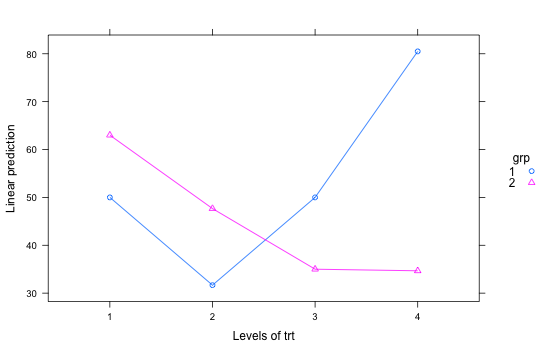
Display these results graphically

> lsmip(dt.lsm, grp ~ trt)

We apparently have different trends for the two groups. Examine the polynomial contrasts

> contrast(dt.lsm, "poly")
grp = 1:
 contrast    estimate        SE df t.ratio p.value
 linear    109.833333 12.621207 13   8.702  <.0001
 quadratic  48.833333  5.644375 13   8.652  <.0001
 cubic     -24.500000 12.621207 13  -1.941  0.0742

grp = 2:
 contrast    estimate        SE df t.ratio p.value
 linear    -97.666667 12.494358 13  -7.817  <.0001
 quadratic  15.000000  5.354725 13   2.801  0.0150
 cubic       9.666667 11.428989 13   0.846  0.4130

These results suggest that we need a quadratic fit but may be able to do without the cubic trends. So let's try a quadratic model:

> dt.poly = lm(resp ~ (trtnum + I(trtnum^2)) * grp, data = dt)
> anova(dt.lm, dt.poly)
Analysis of Variance Table

Model 1: resp ~ trt * grp
Model 2: resp ~ (trtnum + I(trtnum^2)) * grp
  Res.Df   RSS Df Sum of Sq      F Pr(>F)
1     13 248.5                           
2     15 334.2 -2   -85.705 2.2418 0.1457

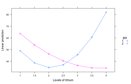
The comparison of the two models is non-significant, so I'll choose the quadratic model as being more parsimonious. Here's the plot

> lsmip(dt.poly, grp ~ trtnum, at = list(trtnum = seq(1, 4, by = .5)))

Obtain the equations of the two parabolas

> summary(dt.poly)

Call:
lm(formula = resp ~ (trtnum + I(trtnum^2)) * grp, data = dt)

Residuals:
    Min      1Q  Median      3Q     Max 
-5.6067 -3.2520 -0.1951  1.2927  9.4100 

Coefficients:
                  Estimate Std. Error t value Pr(>|t|)    
(Intercept)       88.83000    7.99653  11.109 1.23e-08 ***
trtnum           -52.50833    7.49433  -7.006 4.23e-06 ***
I(trtnum^2)       12.69833    1.49887   8.472 4.22e-07 ***
grp2              -0.04951   11.82550  -0.004 0.996715    
trtnum:grp2       23.62622   10.61939   2.225 0.041862 *  
I(trtnum^2):grp2  -8.88939    2.08080  -4.272 0.000668 ***
---
Signif. codes:  0 ‘***’ 0.001 ‘**’ 0.01 ‘*’ 0.05 ‘.’ 0.1 ‘ ’ 1

Residual standard error: 4.72 on 15 degrees of freedom
Multiple R-squared:  0.928, Adjusted R-squared:  0.9041 
F-statistic: 38.69 on 5 and 15 DF,  p-value: 4.723e-08

Thus, the fitted parabolas are:

• Group 1: $\hat y = 88.83 - 52.51 t + 12.70 t^2$
• Group 2: $\hat y = (88.83 - .05) + (-52.51 + 23.63) t + (12.70 - 8.89) t^2 = 88.78 - 31.89 t + 3.81 t^2$