Linear Ridge not correct prediction/coefficients- Scikit learn

Question

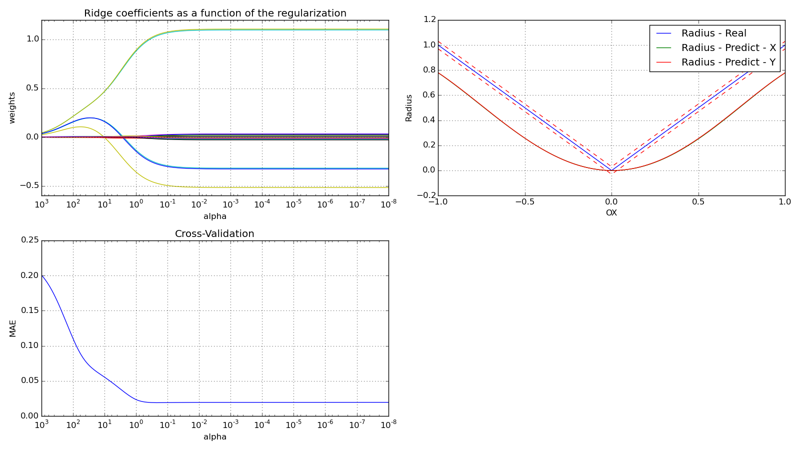
I am using a similar code to this ridge example.

The code proposed is simple. X and Y points inside [-1,1] range and predict the radius creating polynomial features and ridge linear regression.

As the radius is $\sqrt{X^2+Y^2},$ it fits the coefficients of the polynomial to try to simulate a function similar to this one. The thing is that the mean absolute error (MAE) that achieves is very small (~0.03), and when I check the real values and predicted the plot shows that the error has to be much higher.

So it seems that the coefficients are not correct or the MAE it is not correctly calculated.

The code used is the following one:

import numpy as np
import matplotlib.pyplot as plt
from sklearn import linear_model
from sklearn import preprocessing
from sklearn import cross_validation

# Train set
points = np.random.uniform(low=-1.0, high=1.0, size=(100,2))
X = points
y = np.sqrt(X[:,0]**2 + X[:,1]**2)
numRow,numCol = np.shape(X)

# Cross validation
kf = cross_validation.KFold(numRow, n_folds=int(numRow/10))

# Preprocessing
poly = preprocessing.PolynomialFeatures(degree=5, interaction_only=False)
X = poly.fit_transform(X)
print 'Poly: ', poly.powers_, np.shape(poly.powers_)

########################################################################
# Compute paths

n_alphas = 200
alphas = np.logspace(-8, 3, n_alphas)
clf = linear_model.Ridge()

coefs = []
mae = []
for idAlpha,a in enumerate(alphas):

    mae_kFold = np.zeros(len(kf))

    for idKfold,(train_index,test_index) in enumerate(kf):
        X_train, X_test = X[train_index], X[test_index]
        y_train, y_test = y[train_index], y[test_index]

        clf.set_params(alpha=a)
        clf.fit(X_train, y_train)

        y_pred = clf.predict(X_test)
        mae_kFold[idKfold] = np.sum(np.fabs(y_test - y_pred)) / len(y_test)     # MAE (Mean Absolute Error)

        if(idAlpha == 0 and idKfold == 0):
            X_train_3D = X_train
            y_train_3D = y_train
            X_test_3D = X_test
            y_test_3D = y_test
            y_pred_3D = y_pred

    coefs.append(clf.coef_)
    mae.append(np.mean(mae_kFold))


np.set_printoptions(precision=3,suppress=True)
print 'Alpha: ', alphas[0]
print 'Coeff: ', coefs[0], np.shape(coefs[0])
print 'MAE: ', mae[0]

###############################################################################
# Display results

fig = plt.figure(figsize=(16.0,9.0), dpi=100) 

# Subplot 1
plt.subplot(2,2,1)
ax = plt.gca()
ax.set_color_cycle(['b', 'r', 'g', 'c', 'k', 'y', 'm'])

plt.plot(alphas, coefs)
plt.xscale('log')
plt.xlim(ax.get_xlim()[::-1])  # reverse axis
plt.xlabel('alpha')
plt.ylabel('weights')
plt.grid()
plt.title('Ridge coefficients as a function of the regularization')

# Subplot 2
plt.subplot(2,2,2)
OX = np.linspace(-1,1,np.shape(points)[0])
OXY = np.zeros(np.shape(points))
OXY[:,0] = OX
OXY1 = poly.transform(OXY) * coefs[0]
OXY2 = poly.transform(OXY[:,::-1]) * coefs[0]
print 'OXY: ', OXY[:5,:], np.shape(OXY)


plt.plot(OX, np.sqrt(OX**2), label='Radius - Real')
plt.plot(OX, np.sqrt(OX**2)+0.03, 'r--')
plt.plot(OX, np.sqrt(OX**2)-0.03, 'r--')
plt.plot(OX, np.sum(OXY1,axis=1), label='Radius - Predict - X')
plt.plot(OX, np.sum(OXY2,axis=1), label='Radius - Predict - Y')
plt.xlabel('OX')
plt.ylabel('Radius')
plt.grid()
plt.legend()

# Subplot 3
plt.subplot(2,2,3)
ax = plt.gca()
plt.plot(alphas, mae)
plt.xscale('log')
plt.xlim(ax.get_xlim()[::-1])  # reverse axis
plt.xlabel('alpha')
plt.ylabel('MAE')
plt.grid()
plt.title('Cross-Validation')

plt.tight_layout()
plt.show()

Is it a bug or am I doing something wrong?

*CV is not really necessary as results are similar due to random uniform distribution, which works very well for this example.

EDIT

I modified the code slightly to add the prediction results in a 3D view at the end and the predicted values are very close to the real ones so the MAE accuracy (~0.03) is correctly calculated.

# 3D plot

from mpl_toolkits.mplot3d import Axes3D

fig = plt.figure(figsize=plt.figaspect(1))  # Square figure
ax = fig.add_subplot(111, projection='3d')

ax.scatter(X_train_3D[:,1], X_train_3D[:,2], y_train_3D, c='r', s=10, marker="o", lw = 0, alpha=1.0, label='train')
ax.scatter(X_test_3D[:,1], X_test_3D[:,2], y_test_3D, c='g', s=30, marker="o", lw = 0, alpha=1.0, label='test')
ax.scatter(X_test_3D[:,1], X_test_3D[:,2], y_pred_3D, c='b', s=30, marker="o", lw = 0, alpha=1.0, label='pred')

ax.set_xlabel('X axis')
ax.set_ylabel('Y axis')
ax.set_zlabel('Z axis')
plt.legend()

plt.show()

So, the coefficients are wrong! Which one could be the problem?

Answer 1

Quoting from the discussion here: https://github.com/scikit-learn/scikit-learn/issues/5145

When computing the predictions for your plot, you forgot to add the intercept_.