6
$\begingroup$

I understand that you have to run the resulting regression line through the logistic function to get the predicted probability:

am.glm <- glm(am ~ hp + wt, data=mtcars, family=binomial)
newdata <- data.frame(hp=120, wt=2.8)
p1 <- predict(am.glm, newdata, type="response") 
p2 <- 1/(1+exp(-(am.glm$coefficients[1] +
             am.glm$coefficients[2]*newdata[1,1] + 
                 am.glm$coefficients[3]*newdata[1,2])))
p1 - p2
##            1 
## 1.110223e-16

Now I want to build two scoring model with the aim in mind to be usable with a hand calculator only:

  1. First model: I want to just take the two variables ($hp$, $wt$), multiply them by some factor and add them. The resulting number should be compared to a threshold number which then gives me the decision.
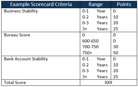
  2. Second model: I want to have certain ranges of the two variables. Depending on the range the variable falls into I am given a number. At the end I simply add all numbers to arrive at my threshold number which again gives me the decision.

As an example from the area of credit scoring where these scorecards are used quite heavily (source: https://www.eflglobal.com/insights-sbbns-credit-risk-problem-loan-management-workshop/):

enter image description here

enter image description here

My question
How to go about and esp. how to transform the logistic regression coefficients to be able to build the two (or any of the two) models?

Perhaps you can even demonstrate the steps in R, making use of the above mtcars logistic regression.

$\endgroup$
4
  • 1
    $\begingroup$ (1) Express the threshold in log odds rather than probability. (2) You need to describe how that scorecard's arrived at. I suspect it's by fitting a different model to yours, in which the predictors are binned & coefficients estimated for each bin. $\endgroup$
    – Scortchi
    Commented Oct 6, 2015 at 8:59
  • $\begingroup$ @Scortchi: So basically if one wants to have a probability of $.5$ the threshold is $exp(.5)/(1-exp(.5)) = -2.54$ ? $\endgroup$
    – vonjd
    Commented Oct 6, 2015 at 9:25
  • $\begingroup$ No - use the logit function, whose inverse is in your code above. The logit of 0.5 is 0. $\endgroup$
    – Scortchi
    Commented Oct 6, 2015 at 9:30
  • 1
    $\begingroup$ @Scortchi: Yeah, silly mistake, so it is $log(.5/(1-.5)) = log(1) = 0$ $\endgroup$
    – vonjd
    Commented Oct 6, 2015 at 9:40

1 Answer 1

2
$\begingroup$

The basic ideas are not that difficult:

  1. First model: You just multiply the respective coefficients with the new data points and see whether the sum is bigger than the negative intercept (then am is 1)
  2. Second model: You first bin the numerical variables into distinct intervals (with cut()) and then run the logistic regression again (dummy variables will be created automatically) . For new data points you check into which interval they would fall and add the resulting coefficients (if the interval is not present you assign 0). You again check whether the sum is bigger than the negative intercept (see first model above).

You can scale all the coefficients and the intercept by multiplying with a factor (e.g. it is quite popular to take 20/ln(2))

As an example consider the following case where we want to build a toy scoring model for predicting am from the mtcars dataset:

library(OneR) # for bin and eval_model function
mtcars_bin <- bin(mtcars)
m <- glm(am ~ hp + wt, data = mtcars_bin, family = binomial)
## Warning: glm.fit: fitted probabilities numerically 0 or 1 occurred
coefficients(m) #points for ranges
##   (Intercept)   hp(109,165]   hp(165,222]   hp(222,278]   hp(278,335] 
##      21.30781      19.62427      19.91155      40.03050      62.28971 
##  wt(2.3,3.08] wt(3.08,3.86] wt(3.86,4.64] wt(4.64,5.43] 
##     -20.61467     -62.03146     -62.78544     -81.47841
prediction <- round(predict(m, type = 'response', mtcars_bin))
eval_model(prediction, mtcars_bin$am)
## 
## Confusion matrix (absolute):
##           Actual
## Prediction  0  1 Sum
##        0   18  1  19
##        1    1 12  13
##        Sum 19 13  32
## 
## Confusion matrix (relative):
##           Actual
## Prediction    0    1  Sum
##        0   0.56 0.03 0.59
##        1   0.03 0.38 0.41
##        Sum 0.59 0.41 1.00
## 
## Accuracy:
## 0.9375 (30/32)
## 
## Error rate:
## 0.0625 (2/32)
## 
## Error rate reduction (vs. base rate):
## 0.8462 (p-value = 1.452e-05)
##
## different scaling
coefficients(m) * 20/log(2)
##   (Intercept)   hp(109,165]   hp(165,222]   hp(222,278]   hp(278,335] 
##      614.8136      566.2367      574.5260     1155.0360     1797.3012 
##  wt(2.3,3.08] wt(3.08,3.86] wt(3.86,4.64] wt(4.64,5.43] 
##     -594.8136    -1789.8496    -1811.6048    -2350.9701

Obviously this model can be further improved by cutting the intervals differently, e.g. combining the ones which give comparable scores, rounding etc., but the general principle stays the same.

$\endgroup$

Your Answer

By clicking “Post Your Answer”, you agree to our terms of service and acknowledge you have read our privacy policy.

Not the answer you're looking for? Browse other questions tagged or ask your own question.