13
$\begingroup$

I am currently reading up on t-SNE visualization technique and it was mentioned that one of the drawbacks of using principal component analysis (PCA) for visualizing high-dimensional data is that it only preserves large pairwise distances between the points. Meaning points which are far apart in high-dimensional space would also appear far apart in low-dimensional subspace but other than that all other pairwise distances would get screwed up.

Could someone help me understand why is that and what does it mean graphically?

$\endgroup$
2
  • $\begingroup$ PCA is closely related to Euclidian and Mahalanobis distances, which are myopic in higher dimensions, they can't see small distances. $\endgroup$
    – Aksakal
    Commented Oct 13, 2015 at 15:33
  • $\begingroup$ Note also that PCA, as seen as simplest metric MDS, is about reconstructing summed squared euclidean distances. Hense, precision for small distances suffers. $\endgroup$
    – ttnphns
    Commented Oct 13, 2015 at 15:36

1 Answer 1

11
$\begingroup$

Consider the following dataset:
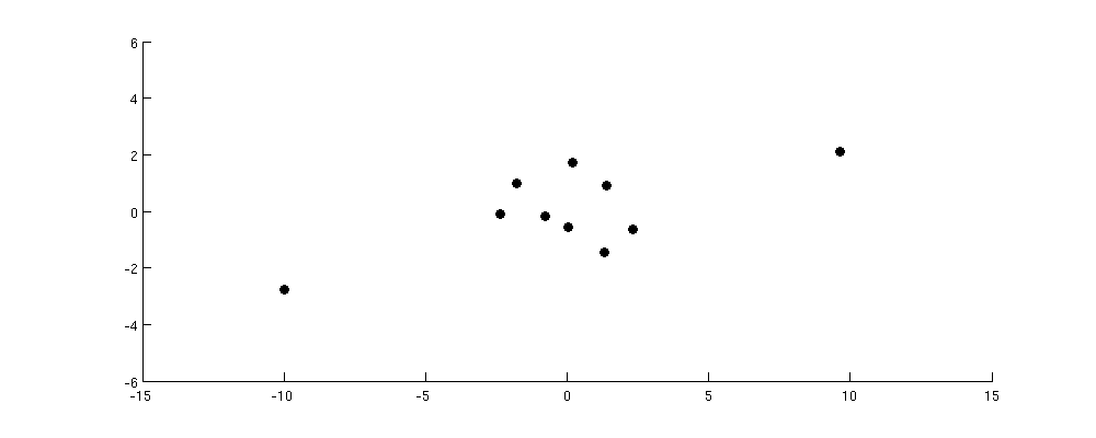
PCA dataset

PC1 axis is maximizing the variance of the projection. So in this case it will obviously go diagonally from lower-left to upper-right corner:
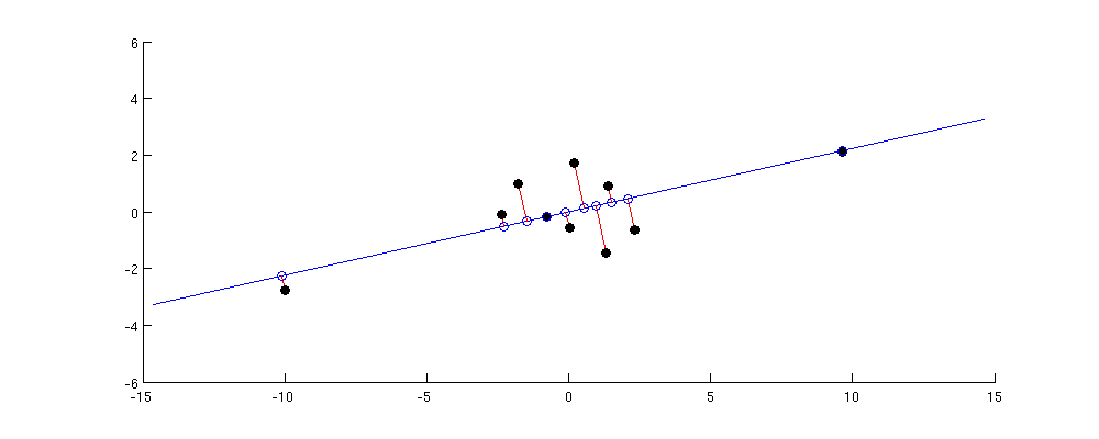
PCA preserving only large pairwise distances

The largest pairwise distance in the original dataset is between these two outlying points; notice that it is almost exactly preserved in the PC1. Smaller but still substantial pairwise distances are between each of the outlying points and all other points; those are preserved reasonably well too. But if you look at the even smaller pairwise distances between the points in the central cluster, then you will see that some of them are strongly distorted.

I think this gives the right intuition: PCA finds low-dimensional subspace with maximal variance. Maximal variance means that the subspace will tend to be aligned such as to go close to the points lying far away from the center; therefore the largest pairwise distances will tend to be preserved well and the smaller ones less so.

However, note that this cannot be turned into a formal argument because in fact it is not necessarily true. Take a look at my answer in What's the difference between principal component analysis and multidimensional scaling? If you take the $10$ points from the figures above, construct a $10\times 10$ matrix of pairwise distances and ask what is the 1D projection that preserves the distances as close as possible, then the answer is given by MDS solution and is not given by PC1. However, if you consider a $10\times 10$ matrix of pairwise centered scalar products, then it is in fact best preserved precisely by PC1 (see my answer there for the proof). And one can argue that large pairwise distances usually mean large scalar products too; in fact, one of the MDS algorithms (classical/Torgerson MDS) is willing to explicitly make this assumption.

So to summarize:

  1. PCA aims at preserving the matrix of pairwise scalar products, in the sense that the sum of squared differences between the original and reconstructed scalar products should be minimal.
  2. This means that it will rather preserve the scalar products with largest absolute value and will care less about those with small absolute value, as they add less towards the sum of squared errors.
  3. Hence, PCA preserves larger scalar products better than the smaller ones.
  4. Pairwise distances will be preserved only as much as they are similar to the scalar products which is often but not always the case. If it is the case, then larger pairwise distances will also be preserved better than the smaller ones.
$\endgroup$
8
  • $\begingroup$ I don't think this is a right visual. It doesn't show how things get worse with dimensionality increase $\endgroup$
    – Aksakal
    Commented Oct 13, 2015 at 21:12
  • 2
    $\begingroup$ I am not sure I understand your point, @Aksakal. Consider posting an alternative answer with your point of view. I think the effect of better preserving larger than smaller pairwise distances is present already in 2D, and one does not need to think about high dimensionality to understand what's going on. Hence I focused on a simple 2D example. $\endgroup$
    – amoeba
    Commented Oct 13, 2015 at 21:22
  • $\begingroup$ What you drew would be applicable to any method. I can put a couple of points very far away and argue that they overweigh the rest. The problem with Euclidian distances is that their dynamic range shrinks with dimensionality increase $\endgroup$
    – Aksakal
    Commented Oct 13, 2015 at 21:30
  • $\begingroup$ +1, But I'd shift an accent, somewhat differently than you did (point 4 mostly). The thing is not that these are distances and those are scalar products (the "double-centration" matrix) - after all, given the diagonal they preserve identical information. Rather, the problem is exactly analogous to the PCA vs Factor analysis odds. Torgerson's PCoA, as PCA, will aim to maximize the reconstruction of the sc. prod. matrix mostly via its diagonal, not controlling specifically how the off-diagonal entries will get fitted. $\endgroup$
    – ttnphns
    Commented Oct 13, 2015 at 22:50
  • $\begingroup$ (cont.) The trace of the mentioned diagonal is the overall variability and is directly related to the sum of all the squared pairwise distances, leaving individual distances behind. It could be phrased also in terms of Eckart-Young theorem which states that PCA-reconstructed data cloud is most close in terms to sum of squares to the original one; that is, the overall squared distance between the old points and their PCA-projected spots is minimal. This is not the same as old pairwise distances - new pw distances relations. $\endgroup$
    – ttnphns
    Commented Oct 13, 2015 at 22:59

Your Answer

By clicking “Post Your Answer”, you agree to our terms of service and acknowledge you have read our privacy policy.

Not the answer you're looking for? Browse other questions tagged or ask your own question.