Calculating integral with antithetic variables

Question

Use simulation with antithetic variables to find

$$\int_{-\infty}^{\infty} \int_0^\infty\, \sin(x+y)e^{-x^2+4x-y}\,dx\,dy.$$ My question is, how struggle with the infinite limit?

It is easy for me to solve similar problems like $\int_0^1e^x\,dx$, but I do not know how to do the stated one.

Answer 1

Overview

The method of antithetic variables is a way to increase the precision of a Monte-Carlo estimate of an integral by finding a way to balance the large values with equally likely small values. The resulting negative correlation reduces the variance of the estimate.

One context in which this tends to work concerns finding expectations. A Monte-Carlo method to find the expectation of any function $g$ of a random variable $X$ is to draw a sequence of independent realizations $x_1, x_2, \ldots, x_n$ according to the probability law $F$ of $X$ and simply average the value of $g$ at these points:

$$\mathbb{E}(g(X)) = \int_\mathbb{R} g(x) dF(x) \approx \frac{1}{n}\sum_{i=1}^n g(x_i).$$

Often, especially for continuous distributions, the desired balance of large against small values can be achieved by pairing each $x_i$, with its antithetic value $x_i^{*}$. This is the number having the complementary quantile of $x_i$; that is,

$$F(x_i) + F(x_i^{*}) = 1.$$

This example

We can recognize the germs of probability distribution functions in the terms $\exp(-x^2 + 4 x)$ and $\exp(-y)$ within the integral because

• Each is non-negative and

• Each has a finite integral: $\exp(-x^2 + 4x) = \exp(-(x-2)^2)\exp(4)$ over the entire set of real numbers, which evaluates to $\exp(4)\sqrt{\pi}$, and $\exp(-y)$ over the positive real numbers, which evaluates to $1$.

This suggests rewriting the integral as

$$\int_0^\infty \int_{-\infty}^{\infty} \sin(x+y) \exp(-x^2 + 4x - y) \mathrm{dx\, dy} = \exp(4)\sqrt{\pi}\,\mathbb{E}(\sin(X+Y))$$

where $X$ has a Normal$(2, \sqrt{1/2})$ distribution and $Y$ has an Exponential distribution.

One step of the numerical integration, then, could proceed as follows:

1. Draw uniform$(0,1)$ random variables $U, V$ independently.

2. Compute the $U$ quantile of a Normal$(2, \sqrt{1/2})$ distribution as $X$ and the $1-U$ quantile of that distribution as $X^{*}$.

3. Compute the $V$ quantile of an Exponential distribution as $Y$ and the $1-V$ quantile of that distribution as $Y^{*}$.

4. Compute $g = \sin(X + Y)$ and $g^{*} = \sin(X^{*} + Y^{*})$.

That produces two values for the eventual average that will be used for the numerical estimate of the integral.

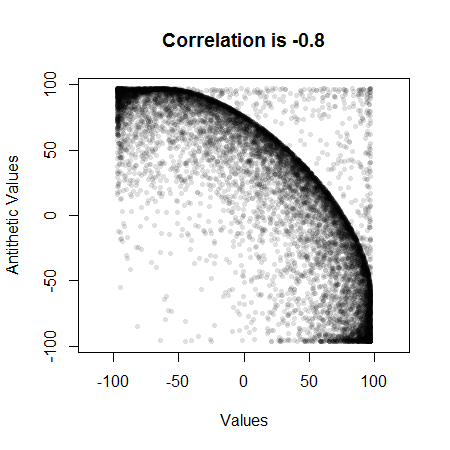
Let's check that this is going to work by computing the correlation between $g$ and $g^{*}$ for a large number of iterations. Here is a plot for $10,000$ iterations:

The large negative correlation indicates this method will work well.

As a fair comparison to a straight Monte-Carlo integration, consider what could be accomplished with $N=1000$ iterations. With antithetic variables we would compute just $N/2=500$ pairs of realizations $(x_i,y_i)$ and use their antithetic counterparts $(x_i^{*}, y_i^{*})$ for the other $500$. Otherwise, we would compute $1000$ sets of $(x_i, y_i)$. Both methods take essentially the same computational effort.

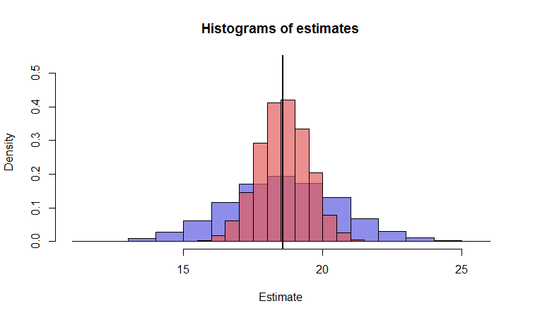
If we were to do this, say, $10,000$ times, we would obtain $10,000$ estimates of the integral with each method. The better method is the one whose estimates range more tightly around the true value. Here are histograms of the two sets of estimates--blue for Monte-Carlo, red for the antithetic version--along with a vertical line locating the value of the integral (at $\exp(15/4)\sqrt{\pi}\,(\cos(2)+\sin(2))/2 \approx 18.5836$.) The superiority of the antithetic method is clear.

The standard deviation of the antithetic method is less than half the SD of the simple method in this case. Equivalently, to achieve any given precision in the estimate requires less than one quarter as much computational effort with the antithetic method (in this example).

Comments

Where did the problem with infinite limits of integration go to? It was handled by the underlying probability distributions.

Note that we can learn about how much better the antithetic method is for any given situation by testing it with a relatively small number of iterations. These results can be used to determine in advance how much computation to devote to the actual calculation.

I implicitly assumed the limits of integration were mixed up in the statement of the problem, for otherwise the integral, as written, diverges.

Code

This R code created the figures. It illustrates how to use the method of antithetic variables. Timing statements confirm that both it and the simple method take the same amount of computational effort.

#
# Compute values of the integrand, given equal-length vectors of uniform 
# variates `u` and `v`.
#
g <- function(u, v) {
  x <- qnorm(u, 2, sqrt(1/2))
  y <- qexp(v)
  exp(4) * sqrt(pi) * sin(x + y)
}
#
# Estimate the integral in two ways, repeatedly.
#
N <- 1e3 / 2
system.time(sim1 <- replicate(1e4, {
  u <- runif(N); v <- runif(N)
  mean(g(c(u, 1-u), c(v, 1-v))) # Antithetical method
}))
system.time(sim2 <- replicate(1e4, {
  u <- runif(2*N); v <- runif(2*N)
  mean(g(u,v))                  # "Simple" method
}))
#
# Plot the histograms of each method.
#
par(mfrow=c(1,1))
hist(sim2, freq=FALSE, breaks=20, ylim=c(0, 0.75*sqrt(N/1000)), col="#5b5be0b0",
     xlab="Estimate", main="Histograms of estimates")
hist(sim1, freq=FALSE, breaks=20, add=TRUE, col="#e05b5bb0")
abline(v = exp(15/4) * sqrt(pi) * (cos(2) + sin(2))/2, lwd=2)
#
# Study the correlation of the antithetic variables.
#
u <- runif(1e4); v <- runif(1e4)
g0 <- g(u, v)
g1 <- g(1-u, 1-v)
plot(g0, g1, asp=1, pch=16, col="#00000020", cex=0.75,
     xlab="Values", ylab="Antithetic Values",
     main=paste("Correlation is", format(cor(g0, g1), digits=2)))

Answer 2

There is no answer to this question because the integral diverges and so numerically you won't get a reliable answer using simulation.

Here is a link to Wolfram to see that the integral diverges: http://www.wolframalpha.com/input/?i=integral_-infty^infty+integral_0^infity+si‌​n%28x%2By%29*e^%28x^2%2B4x-y%29+dx+dy

But since you insist that R says the integral evaluates to 18.58, here is some R code for calculating double integrals that says the contrary.

##############################################################################
###First Solution
############################################################################## 

myfun <- function(x,y) sin(x+y)*exp(x^2+4*x-y)
llim.x <- 0
ulim.x <- Inf

llim.y <- -Inf
ulim.y <- Inf

integrate(function(y) { 
   sapply(y, function(y) {
     integrate(function(x) myfun(x,y), llim.x, ulim.x)$value
   })
 }, llim.y, ulim.y)

##############################################################################
###Second Solution
############################################################################## 

library(pracma)
quad2d(myfun, 0, 1, -1, 1)
quad2d(myfun, 0, 10, -10, 10)
quad2d(myfun, 0, 100, -100, 100)
quad2d(myfun, 0, Inf, -Inf, Inf)

And so you see, in the second method, as you increase the limits to infinity, the solutions blows up to $\infty$.