2
$\begingroup$

I am studying logistic regressions and I wonder why are estimators biased when the independent variables have low variance (maybe low variance compared to its mean, but anyway).

I simulate the underlying model as a linear function of a single variable x and I do not include an error term. x is generated from a normal distribution, with mean mx and sd sx.

f is a helper to map the probabilities using a logistic function

I use mx = 1.0, and sample sx from a uniform distribution from 0 to 1, so I can estimate the model for different values of sx.

SAMPLE_SIZE = 1000
set.seed(100)

f <- function(v) exp(v) / (1 + exp(v));

sim = function(b0, b1, mx, sx) {
  xs <- rnorm(SAMPLE_SIZE, mean = mx, sd = sx)
  ps <- f(b0 + b1 * xs)
  ys <- rbinom(SAMPLE_SIZE, 1, ps)
  glm(ys ~ xs, family = binomial)
}  


sx <- runif(n = 1000, min = 0.05, max = 1.0)
b0 = 1.5
b0s <- sapply(sx, function(v) {
  sim(b0 = b0, b1 = 1.0, mx = 1.0, sx = v)$coefficients[[1]]
})

And then I plot the error between the estimated b0 coefficient and the real one, for different values of sx:

plot(sx, b0s - b0)

What I get is that the error gets smaller the greater sx is.

From common linear regressions, we know that the estimators get more precise the larger the variance in the independent variables. But that does not say anything about the biases.

How to interpret this result? Are the estimators really biased in logistic regressions? What's missing here? Is there any problem related to numerical estimates here?

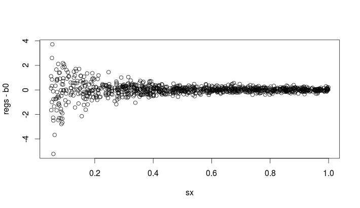
Estimation error vs. standard deviation in X

$\endgroup$
3
  • $\begingroup$ How does this address bias? You plot at the end doesn't seem to indicate any bias. $\endgroup$
    – Dason
    Commented Dec 24, 2015 at 3:33
  • 2
    $\begingroup$ Your plot does demonstrate variance, however... $\endgroup$
    – Sycorax
    Commented Dec 24, 2015 at 5:28
  • $\begingroup$ Hummm it really does not demonstrate bias but does demonstrate variance... Thanks for the answer. @Dason $\endgroup$ Commented Dec 24, 2015 at 5:31

1 Answer 1

2
$\begingroup$

Note that the apparent 'bias' disappears when you make mx=0, as in:

library(txtplot)
f <- function(v) exp(v) / (1 + exp(v));

sim = function(b0, b1, mx, sx, SAMPLE_SIZE=1000) {
  xs <- rnorm(SAMPLE_SIZE, mean = mx, sd = sx)
  ps <- f(b0 + b1 * xs)
  ys <- rbinom(SAMPLE_SIZE, 1, ps)
  glm(ys ~ xs, family = binomial)
}

b0 <- 1.5
b1 <- 1.0
mx <- 1
sx <- seq(from=0.05,to=1.0,by=0.005)
set.seed(100)
b0s <- sapply(sx, function(v) {
  sim(b0 = b0, b1 = b1, mx = mx, sx = v)$coefficients[[1]]
})
#' And then I plot the error between the estimated b0 coefficient and the real one, for different values of sx:
txtplot::txtplot(sx,b0s-b0,width=90)

#'    +---------------+----------------+---------------+---------------+----------------+---+
#'  4 +     *                                                                               +
#'    |                                                                                     |
#'    |                                                                                     |
#'  3 +   *                                                                                 +
#'    |                                                                                     |
#'    |                                                                                     |
#'  2 +                                                                                     +
#'    |                                                                                     |
#'    |   *                                                                                 |
#'    |       *        **                                                                   |
#'  1 +      *  *             *                                                             +
#'    |     *   *   *     ***             *   *                                             |
#'    |           ** *    * *            *  *       *   * **     *                          |
#'  0 +          * *    *    ********* *************** ************** ***** *************   +
#'    |       * *             **** *  **    * **** *  **    ** *  ** **** ** *    *   **    |
#'    |    *   *   *  *  *   *  *   * * *          *                                        |
#'    |      *    * ****    *                                                               |
#' -1 +     * ** *     *                                                                    +
#'    |    *                                                                                |
#'    +---------------+----------------+---------------+---------------+----------------+---+
#'                   0.2              0.4             0.6             0.8               1

# and again, with mx=0
mx <- 0
set.seed(100)
b0s <- sapply(sx, function(v) {
  sim(b0 = b0, b1 = b1, mx = mx, sx = v)$coefficients[[1]]
})
#' And then I plot the error between the estimated b0 coefficient and the real one, for different values of sx:
txtplot::txtplot(sx,b0s-b0,width=90)
#'      +---------------+---------------+---------------+---------------+---------------+---+
#'      |                                                       *                           |
#'      |                                                                                   |
#'  0.2 +                                            *                                      +
#'      |                                 *                 *                               |
#'      |           *       **             * *    *   *              *               *      |
#'      |      *      *                      *    *          *    *                 *       |
#'  0.1 +        *       *   *  *   *    *                           *       *   *  ***     +
#'      |   ***        * *     *     *     **    * **                             *   *     |
#'      |       *   **      **          *     **          *    ***     ***      *           |
#'      |     *   *        *  ** *     *       **     *      **          *    *             |
#'    0 +   *        *  * *    *  ** *   ***    *   *   * **        *        *              +
#'      |       *  *  *               ***        *      **  *      *      * *  *   *        |
#'      |        *   * **  *     *   **  *   *      *  *    * *   **  ***             * *   |
#'      |      *   *                *         *   *  *     *        * * * *   * ***         |
#' -0.1 +                  *  *    *   *                      **            *     *    *    +
#'      |    *   **      **                 *      *    *           *      *   *       **   |
#'      |                                                                 **       *        |
#'      |                                      *                  *             *   *       |
#' -0.2 +                         *                                                         +
#'      +---------------+---------------+---------------+---------------+---------------+---+
#'                     0.2             0.4             0.6             0.8              1

Think about it this way: your independent variable $x$ has mean 1 and standard deviation sx. When sx is very small, $x$ is almost indistinguishable from the constant 1 intercept 'variable', so a logistic regression 'has a hard time' disambiguating the effect of $x$. This is much easier when the variation in $x$ (and thus the resultant variation in the odds of the dependent variable) is larger.

$\endgroup$

Your Answer

By clicking “Post Your Answer”, you agree to our terms of service and acknowledge you have read our privacy policy.

Not the answer you're looking for? Browse other questions tagged or ask your own question.