why cost function needs to be smooth, how this helps in learning?

Question

From what I understand a smooth function 1-degree is a function whose first derivative is continuous? How this helps in estimating the parameters? What if the function is not smooth?

Answer 1

First, the cost function does not to be smooth, and there are many widely used cost functions are not smooth. For example, the loss for least absolute deviations and support vector machine is using Hinge Loss, which is also not smooth.

Here is the comparison for least square and least absolute deviation. Least absolute deviation is widely used and more robust to outliers.

• Least square (smooth) $L(y,\hat y)=(y-\hat y)^2$

• Least absolute deviation(continuous but not smooth) $L(y,\hat y)=|y-\hat y|$

Second, continuous and differentiable (smooth) are good features to have in the cost function (but perfectly OK to not have). If the objective function is smooth, and we can calculate the gradient, the optimization (how to find the values for all parameters) is easier to solve.

Many solvers need gradient as an input. Intuitively, gradient tells us where to go to update parameters to get lower cost in the optimization (model fitting) process. On the other hand, there are many gradient free algorithm to do the optimization, so it is OK to have a non-smooth objective function.

In addtion, in real world, not only the objective function can be non-smooth, but also it can discretely defined. Think about 0-1 loss, which is number of mis-classifications. It is a discrete function, where

$L(y,\hat y)=$ $ \begin{cases} 0 & y=\hat y\\ 1 & y\neq\hat y \end{cases} $ If a function is a discrete function then it definitely is not smooth.

0-1 loss is hard to minimize and we are not directly using it in real world. But the reason is not because it is non-smooth but it is non-convex.

---

Comparing to smoothness, convexity is a more important for cost functions. A convex function is easier to solve comparing to non-convex function regardless the smoothness.

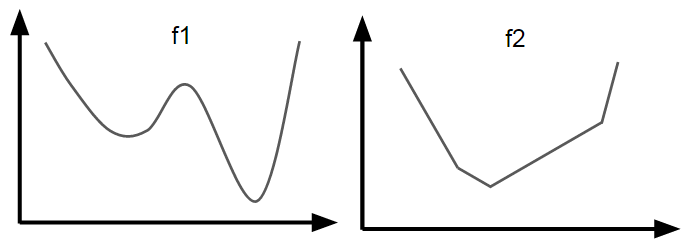
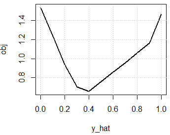
In this example, function 1 is non-convex and smooth, and function 2 is convex and none-smooth. Performing optimization on f2 is much easier than f1. In fact, the loss for least absolute deviations on whole data set is very similar to f2.

Here is code to plot the loss function on a toy data set for least absolute regression. Where in this data set, you only have 3 data points, you only have the target (no features). y_hat is your estimation, and obj is the least absolute loss in whole data.

set.seed(0)
y=runif(3)
y_hat=seq(0,1,0.1)
obj=sapply(y_hat,function(y_hat) sum(abs(y-y_hat)))
plot(y_hat,obj,type="l",lwd=2)
grid()