You can use a random-effects model in place of a paired t-test.
Say you have two sets of measurements denoted by $i=1$ and $i=2$ one of the population mean $\mu_1$ and one of the population mean $\mu_2$. The measurement consists of points $y_{ij}$, which have errors within participants $\epsilon_j$ and from test to test $\epsilon_{ij}$
$$y_{ij} = \mu_i + \epsilon_j + \epsilon_{ij}$$
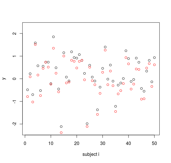
it may look as following for 50 subjects when $\mu_1 = 0.1, \mu_2 = -0.1, \epsilon_j \sim N(0,1), \epsilon_{ij} \sim N(0,0.01)$

The points in this example have a lot of scattering due to the error $\epsilon_j$ related with each individual. The estimates of the means for each separate group would involve large errors. However, the estimate in terms of an intercept term plus a difference term might be well estimated.
- With a paired t-test you use the differences and compute it as a single sample t-test.
- With a mixed-effects model, you estimate the parameter/slope/coefficient for the difference and estimate its standard deviation/error. This estimate is done with the covariance matrix of the errors (which is itself estimated as well). Because this covariance matrix includes terms for the correlation of the measurements within the same subject, you end up with a small standard error in the effect for the difference between the $\mu_i$.
This mixed-effects model can still be used when you do not have all of the data points paired. (see R code example below) Some aspects:
With the mixed-effects model you can express a t-value based on the estimated effect and its estimated standard error. However, there is no straightforward formulation for the related degrees of freedom and the t-distribution that relates to this t-value. But, for significance testing, you could also use a likelihood ratio test.
You could also use a paired test with only the paired points available, but the mixed-effects model is doing slightly better because it will be better able to estimate the group for which you have more points.
To see this intuitively, imagine a worst case when you have a lot of points for both groups (and thus the means of both groups can be estimated accurately) but only a small overlap with the pairing between the points (in which case just using the paired points will reduce the precision).
You can see it work as follows: The error for the paired differences is due to the $\epsilon_{ij}$. By using additional information from the un-paired points you can slightly bias the paired points to get a more precise estimate.
set.seed(1)

### settings
ni <- 50     # group size
nr <- 10     # reduced group size
d = 0.2      # difference in group means
sig <- 0.1   # stdev of sampling error
tau <- 1     # stdev of subjects

### subject error
err_subj <- rnorm(ni, 0 , tau)

### observations
###       mean      + subject effect/error + sampling error
y <- c(rep(d/2,ni)  + err_subj             + rnorm(ni,0,sig),
       rep(-d/2,ni) + err_subj             + rnorm(ni,0,sig))
### regressors (group and subject)
xgroup <-  c(rep(1/2,ni), rep(-1/2,ni))
xgroup2 <- c(rep((ni)/(ni+nr),ni), rep(-(nr)/(ni+nr),ni))
xsubj <- c(c(1:ni),c(1:ni))

### creat data tables
data <- list(y=y,
             xgroup = as.numeric(xgroup),
             xsubj = as.factor(xsubj))
data2 <- list(y=y[-c(1:(ni-nr))],
             xgroup = as.numeric(xgroup[-c(1:(ni-nr))]),
             xsubj = as.factor(xsubj[-c(1:(ni-nr))]))


### perform regression
mod <- lme4::lmer(y ~ 1 + xgroup +  (1|xsubj),  data = data)
mod2 <- lme4::lmer(y ~ 1 + xgroup +  (1|xsubj),  data = data2)
mod3 <- lm(y  ~ 1 + xgroup, data = data2)

### test statistics summary
summary(mod2)
summary(mod3)

### significance test using chi-squared / likelihood-ratio
drop1(mod2,test="Chisq")
drop1(mod3,test="Chisq")

plot(y[c(1:ni)], ylim = c(-2.3,2.3),
     xlab = "subject i", ylab = "y")
points(y[c(1:ni)+ni], col  =2)


