43
$\begingroup$

I want to regress a variable $y$ onto $x,x^2,\ldots,x^5$. Should I do this using raw or orthogonal polynomials? I looked at the question on the site that deals with these, but I don't really understand what's the difference between using them.

Why can't I just do a "normal" regression to get the coefficients $\beta_i$ of $y=\sum_{i=0}^5 \beta_i x^i$ (along with p-values and all the other nice stuff) and instead have to worry whether using raw or orthogonal polynomials? This choice seems to me to be outside the scope of what I want to do.

In the stat book I'm currently reading (ISLR by Tibshirani et al) these things weren't mentioned. Actually, they were downplayed in a way.
The reason is, AFAIK, that in the lm() function in R, using y ~ poly(x, 2) amounts to using orthogonal polynomials and using y ~ x + I(x^2) amounts to using raw ones. But on pp. 116 the authors say that we use the first option because the latter is "cumbersome" which leaves no indication that these commands actually do two completely different things (and have different outputs as a consequence).
(third question) Why would the authors of ISLR confuse their readers like that?

$\endgroup$
9
  • 1
    $\begingroup$ @Sycorax I know that poly has something to do with orthogonal polynomials and I(x^2) doesn't (though I don't know the details) - but still, why would the authors of ISLR then recommend a method that does not work ? It seems very misleading if both command seem to do the same, but only one actually is ok. $\endgroup$
    – l7ll7
    Commented Jan 26, 2017 at 16:15
  • 1
    $\begingroup$ @gung I looked at the documentation of poly and spent already a while with this problem, but I can't figure out why poly(x,2) and x+I(x^2) make a difference? Could you please enlighten me here in the comments, if the question is offtopic? $\endgroup$
    – l7ll7
    Commented Jan 26, 2017 at 16:18
  • 1
    $\begingroup$ @gung I did a completey re-edit of my question. This choice raw/orthogonal is confusing me even more - previously I thought this was just a minor R technicality, that I didn't understand, but now it seems to be a fullblown stat problem that hinders me of doing coding a regression that should not be that difficult to code. $\endgroup$
    – l7ll7
    Commented Jan 26, 2017 at 16:37
  • 3
    $\begingroup$ @gung That actually confused me more than it helped. Previously I thought that I should just go with orthogonal polynomials, because that seemed to be the right way, but in that answer raw polynomials are used. Suprisingly, everyone on the net is screaming "RTFM", but there is actually not clear answer, when to use what. (Your link also doesn't give an answer to this, just an example, when orth. pol. go wrong) $\endgroup$
    – l7ll7
    Commented Jan 27, 2017 at 10:31
  • 3
    $\begingroup$ Unless you are working in some physical or engineering domain that states the response will be a quintic polynomial, almost surely the right approach is not to do polynomial regression in the first place. Invest your degrees of freedom in a spline or something that would be far more flexible and stable than the polynomial fit. $\endgroup$
    – whuber
    Commented Mar 9, 2018 at 21:46

5 Answers 5

34
$\begingroup$

I feel like several of these answers miss the point. Haitao's answer addresses the computational problems with fitting raw polynomials, but it's clear that OP is asking about the statistical differences between the two approaches. That is, if we had a perfect computer that could represent all values exactly, why would we prefer one approach over the other?

user5957401 argues that orthogonal polynomials reduce the collinearity among the polynomial functions, which makes their estimation more stable. I agree with Jake Westfall's critique; the coefficients in orthogonal polynomials represent completely different quantities from the coefficients on raw polynomials. The model-implied dose-response function, $R^2$, MSE, predicted values, and the standard errors of the predicted values will all be identical regardless of whether you use orthogonal or raw polynomials.

The coefficient on $X$ in a raw polynomial regression of order 2 has the interpretation of "the instantaneous change in $Y$ when $X=0$." If you performed a marginal effects procedure on the orthogonal polynomial where $X=0$, you would get exactly the same slope and standard error, even though the coefficient and standard error on the first-order term in the orthogonal polynomial regression are completely different from their values in the raw polynomial regression. That is, when trying to get the same quantities from both regressions (i.e., quantities that can be interpreted the same way), the estimates and standard errors will be identical. Using orthogonal polynomials doesn't mean you magically have more certainty of the slope of $X$ at any given point. The stability of the models is identical.

In the example below, I fit a raw polynomial model and an orthogonal polynomial model on the same data using polynomials of order 3. To get a parameter with the same interpretation as the slope on the second-order (squared) term in the raw model, I used a marginal effects procedure on the orthogonal model, requesting the slope when the predictor is equal to 0.

data("iris")

#Raw:
fit.raw <- lm(Petal.Length ~ Petal.Width + I(Petal.Width^2) +
                  I(Petal.Width^3), data = iris)
summary(fit.raw)

#> Coefficients:
#>                  Estimate Std. Error t value Pr(>|t|)    
#> (Intercept)        1.1034     0.1304   8.464 2.50e-14 ***
#> Petal.Width        1.1527     0.5836   1.975  0.05013 .  
#> I(Petal.Width^2)   1.7100     0.5487   3.116  0.00221 ** 
#> I(Petal.Width^3)  -0.5788     0.1408  -4.110 6.57e-05 ***
#> ---
#> Signif. codes:  0 '***' 0.001 '**' 0.01 '*' 0.05 '.' 0.1 ' ' 1
#> 
#> Residual standard error: 0.3898 on 146 degrees of freedom
#> Multiple R-squared:  0.9522, Adjusted R-squared:  0.9512 
#> F-statistic: 969.9 on 3 and 146 DF,  p-value: < 2.2e-16

#Orthogonal
fit.orth <- lm(Petal.Length ~ stats::poly(Petal.Width, 3), data = iris)

#Marginal effect of X at X=0 from orthogonal model
library(margins)
summary(margins(fit.orth, variables = "Petal.Width", 
                at = data.frame(Petal.Width = 0)))
#> Warning in check_values(data, at): A 'at' value for 'Petal.Width' is
#> outside observed data range (0.1,2.5)!
#>       factor Petal.Width    AME     SE      z      p  lower  upper
#>  Petal.Width      0.0000 1.1527 0.5836 1.9752 0.0482 0.0089 2.2965

Created on 2019-10-25 by the reprex package (v0.3.0)

The marginal effect of Petal.Width at 0 from the orthogonal fit and its standard error are exactly equal to those from the raw polynomial fit (i.e., 1.1527). Using orthogonal polynomials doesn't improve the precision of estimates of the same quantity between the two models.

The key is the following: using orthogonal polynomials allows you to isolate the contribution of each term to explaining variance in the outcome, e.g., as measured by the squared semipartial correlation. If you fit an orthogonal polynomial of order 3, the squared semipartial correlation for each term represents the variance in the outcome explained by that term in the model. So, if you wanted to answer "How much of the variance in $Y$ is explained by the linear component of $X$?" you could fit an orthogonal polynomial regression, and the squared semipartial correlation on the linear term would represent this quantity. This is not so with raw polynomials. If you fit a raw polynomial model of the same order, the squared partial correlation on the linear term does not represent the proportion of variance in $Y$ explained by the linear component of $X$. See below.

library(jtools)
data("iris")

fit.raw3 <- lm(Petal.Length ~ Petal.Width + I(Petal.Width^2) +
                  I(Petal.Width^3), data = iris)
fit.raw1 <- lm(Petal.Length ~ Petal.Width, data = iris)

round(summ(fit.raw3, part.corr = T)$coef, 3)
#>                    Est.  S.E. t val.     p partial.r part.r
#> (Intercept)       1.103 0.130  8.464 0.000        NA     NA
#> Petal.Width       1.153 0.584  1.975 0.050     0.161  0.036
#> I(Petal.Width^2)  1.710 0.549  3.116 0.002     0.250  0.056
#> I(Petal.Width^3) -0.579 0.141 -4.110 0.000    -0.322 -0.074

round(summ(fit.raw1, part.corr = T)$coef, 3)
#>              Est.  S.E. t val. p partial.r part.r
#> (Intercept) 1.084 0.073 14.850 0        NA     NA
#> Petal.Width 2.230 0.051 43.387 0     0.963  0.963

fit.orth3 <- lm(Petal.Length ~ stats::poly(Petal.Width, 3), 
               data = iris)
fit.orth1 <- lm(Petal.Length ~ stats::poly(Petal.Width, 3)[,1], 
               data = iris)

round(summ(fit.orth3, part.corr = T)$coef, 3)
#>                                Est.  S.E.  t val. p partial.r part.r
#> (Intercept)                   3.758 0.032 118.071 0        NA     NA
#> stats::poly(Petal.Width, 3)1 20.748 0.390  53.225 0     0.975  0.963
#> stats::poly(Petal.Width, 3)2 -3.015 0.390  -7.735 0    -0.539 -0.140
#> stats::poly(Petal.Width, 3)3 -1.602 0.390  -4.110 0    -0.322 -0.074

round(summ(fit.orth1, part.corr = T)$coef, 3)
#>                                    Est.  S.E. t val. p partial.r part.r
#> (Intercept)                       3.758 0.039 96.247 0        NA     NA
#> stats::poly(Petal.Width, 3)[, 1] 20.748 0.478 43.387 0     0.963  0.963

Created on 2019-10-25 by the reprex package (v0.3.0)

The squared semipartial correlations for the raw polynomials when the polynomial of order 3 is fit are $0.001$, $0.003$, and $0.005$. When only the linear term is fit, the squared semipartial correlation is $0.927$. The squared semipartial correlations for the orthogonal polynomials when the polynomial of order 3 is fit are $0.927$, $0.020$, and $0.005$. When only the linear term is fit, the squared semipartial correlation is still $0.927$. From the orthogonal polynomial model but not the raw polynomial model, we know that most of the variance explained in the outcome is due to the linear term, with very little coming from the square term and even less from the cubic term. The raw polynomial values don't tell that story.

Now, if you want this interpretational benefit over the interpretational benefit of actually being able to understand the coefficients of the model, then you should use orthogonal polynomials. If you would prefer to look at the coefficients and know exactly what they mean (though I doubt one typically does), then you should use the raw polynomials. If you don't care (i.e., you only want to control for confounding or generate predicted values), then it truly doesn't matter; both forms carry the same information with respect to those goals. I would also argue that orthogonal polynomials should be preferred in regularization (e.g., lasso), because removing higher-order terms doesn't affect the coefficients of the lower order terms, which is not true with raw polynomials, and regularization techniques often care about the size of each coefficient.

$\endgroup$
7
  • 1
    $\begingroup$ Excellent contribution. I can't replicate your marginal results (the margin function pops an error about poly when I try to run your first block of code -- I'm not familiar with the margin package) -- but they are exactly what I expect. As a small suggestion -- you should include the output of the margin analysis on the raw model as well. Your argument is undermined (slightly) by the change in p-values from the summary to the margin functions (changing our conclusions no less!) -- which seems to be caused by using a normal instead of a t distribution. Your regularization point is excellent. $\endgroup$ Commented Nov 14, 2019 at 22:13
  • 1
    $\begingroup$ Thank you for the kind words. I think you have to include the stats:: in the call to poly() in lm() for margins to recognize it (which is stupid). I wanted to focus my argument on the point estimates and standard errors, and I know there is a lot of extraneous and distracting information presented, but I hope the text illustrates my points. $\endgroup$
    – Noah
    Commented Nov 15, 2019 at 4:28
  • 1
    $\begingroup$ @skan it doesn't matter. Both will give you identical predicted values of Y for each value of X with the same standard error. For computational reasons it might be better to use orthogonal, especially if you are dealing with very large or very small values. $\endgroup$
    – Noah
    Commented Jul 5, 2022 at 18:55
  • 1
    $\begingroup$ @Noah. I understand what are X and X^2 in a regular model, and how to interpret the coefficients. But what are X and X^2 in a model that has been orthogonalized by poly()? $\endgroup$
    – skan
    Commented Jul 6, 2022 at 18:48
  • 2
    $\begingroup$ @skan The coefficients on the orthogonal polynomials are uninterpretable. I would argue that understanding what $X^2$ means doesn't mean you know what the coefficient on $X^2$ means, but maybe you do (I wouldn't attempt to interpret it). If your goal is prediction rather than interpretation of the coefficients in your model, does it really matter? If you want to understand the relationship between X and Y, plotting it is better than trying to read coefficients, and the plot will be the same whether you use raw or orthogonal polynomials. $\endgroup$
    – Noah
    Commented Jul 6, 2022 at 19:24
18
$\begingroup$

I believe the answer is less about numeric stability (though that plays a role) and more about reducing correlation.

In essence -- the issue boils down to the fact that when we regress against a bunch of high order polynomials, the covariates we are regressing against become highly correlated. Example code below:

x = rnorm(1000)
raw.poly = poly(x,6,raw=T)
orthogonal.poly = poly(x,6)
cor(raw.poly)
cor(orthogonal.poly)

This is tremendously important. As the covariates become more correlated, our ability to determine which are important (and what the size of their effects are) erodes rapidly. This is typically referred to as the problem of multicollinearity. At the limit, if we had two variables that were fully correlated, when we regress them against something, its impossible to distinguish between the two -- you can think of this as an extreme version of the problem, but this problem affects our estimates for lesser degrees of correlation as well. Thus in a real sense -- even if numerical instability wasn't a problem -- the correlation from higher order polynomials does tremendous damage to our inference routines. This will manifest as larger standard errors (and thus smaller t-stats) that you would otherwise see (see example regression below). For this reason, we might choose to orthogonalize our polynomials before regressing them.

y = x*2 + 5*x**3 - 3*x**2 + rnorm(1000)
raw.mod = lm(y~poly(x,6,raw=T))
orthogonal.mod = lm(y~poly(x,6))
summary(raw.mod)
summary(orthogonal.mod)

If you run this code, interpretation is a touch hard because the coefficients all change and so things are hard to compare. Looking at the T-stats though, we can see that the ability to determine the coefficients was MUCH larger with orthogonal polynomials. For the 3 relevant coefficients, I got t-stats of (560,21,449) for the orthogonal model, and only (28,-38,121) for the raw polynomial model. This is a huge difference for a simple model with only a few relatively low order polynomial terms that mattered.

That is not to say that this comes without costs. There are two primary costs to bear in mind. 1) we lose some interpretability with orthogonal polynomials. We might understand what the coefficient on x**3 means, but interpreting the coefficient on x**3-3x (the third hermite poly -- not necessarily what you will use) can be much harder. Second -- when we say that these are polynomials are orthogonal -- we mean that they are orthogonal with respect to some measure of distance. Picking a measure of distance that is relevant to your situation can be difficult. However, having said that, I believe that the poly function is designed to choose such that it is orthogonal with respect to covariance -- which is useful for linear regressions.

$\endgroup$
5
  • 6
    $\begingroup$ -1. The larger standard errors that you see on the lower order coefficients is a red herring. The lower order coefficients in your two models are estimating completely different things, so comparing their standard errors makes no sense. The highest order coefficient is the only one estimating the same thing in both models, and you'll see that the t statistic is identical whether the polynomials are orthogonal or not. Your two models are statistically equivalent in terms of fitted values, R^2, etc., they differ mainly just in interpretation of the coefficients $\endgroup$ Commented Oct 24, 2019 at 16:38
  • $\begingroup$ @JakeWestfall, I don't think I agree with you. First of all, running the code produces values which are different for all of the polynomial orders, not all but one -- in essence it takes the polynomial and does PCA on it. Secondly, and more importantly, the t-stats are substantially different -- running the code in my answer will confirm that -- functionally we are solving the multicollinearity problem. You are right that fitted values, R^2, F-tests etc don't change. That in fact is a reason to orthogonalize -- it changes nothing except our ability to detect polynomial terms. $\endgroup$ Commented Oct 25, 2019 at 18:05
  • 1
    $\begingroup$ Re: the first point, sorry, I meant to refer to the t-stat of the highest-order term, not its coefficient. That predictor is scaled+shifted between models, so yes the coef changes, but it tests the same substantive effect, as shown by t $\endgroup$ Commented Oct 25, 2019 at 19:46
  • 1
    $\begingroup$ Re: the second point, the reason "the t-stats are substantially different" for the lower-order terms is, again, because they are estimating completely different things in the two models. Consider the linear effect: in raw.mod it estimates the slope of the curve at x=0, in orthogonal.mod it estimates the marginal slope (i.e., identical to lm(y ~ poly(x,1)) where higher-order terms are omitted). There is no reason that estimates of these completely different estimands should have comparable standard errors. One can easily construct a counter-example where raw.mod has much higher t-stats $\endgroup$ Commented Oct 25, 2019 at 19:48
  • 1
    $\begingroup$ @JakeWestfall. I still think you're missing the multicollinearity. However, we seem to be talking past each other, and there is perhaps a solution. You say you can easily construct a counter-example, please do. I think seeing the dgp you have in mind would clarify a lot for me. At the moment the only things I've been able to come up with which might behave as you describe involve severe model misspecification. $\endgroup$ Commented Oct 29, 2019 at 18:26
12
$\begingroup$

Why can't I just do a "normal" regression to get the coefficients?

Because it is not numerically stable. Remember computer is using fixed number of bits to represent a float number. Check IEEE754 for details, you may surprised that even simple number $0.4$, computer need to store it as $0.4000000059604644775390625$. You can try other numbers here

Using raw polynomial will cause problem because we will have huge number. Here is a small proof: we are comparing matrix condition number with raw and orthogonal polynomial.

> kappa(model.matrix(mpg~poly(wt,10),mtcars))
[1] 5.575962
> kappa(model.matrix(mpg~poly(wt,10, raw = T),mtcars))
[1] 2.119183e+13

You can also check my answer here for an example.

Why are there large coefficents for higher-order polynomial

$\endgroup$
1
  • 8
    $\begingroup$ You seem to be using single precision floats and quoting them to quadruple precision! How did that happen? Except for GPUs, almost all statistical computation uses at least double precision. E.g., in R the output of print(0.4, digits=20) is 0.40000000000000002. $\endgroup$
    – whuber
    Commented Mar 9, 2018 at 21:43
2
$\begingroup$

I would have just commented to mention this, but I do not have enough rep, so I'll try to expand into an answer. You might be interested to see that in Lab Section 7.8.1 in "Introduction to Statistical Learning" (James et. al., 2017, corrected 8th printing), they do discuss some differences between using orthogonal polynomials or not, which is using the raw=TRUE or raw=FALSE in the poly() function. For example, the coefficient estimates will change, but the fitted values do not:

# using the Wage dataset in the ISLR library
fit1 <- lm(wage ~ poly(age, 4, raw=FALSE), data=Wage)
fit2 <- lm(wage ~ poly(age, 4, raw=TRUE), data=Wage)
print(coef(fit1)) # coefficient estimates differ
print(coef(fit2))
all.equal(predict(fit1), predict(fit2)) #returns TRUE    

The book also discusses how when orthogonal polynomials are used, the p-values obtained using the anova() nested F-test (to explore what degree polynomial might be warranted) are the same as those obtained when using the standard t-test, output by summary(fit). This illustrates that the F-statistic is equal to the square of the t-statistic in certain situations.

$\endgroup$
2
  • $\begingroup$ Comments should never be used as answers regardless of your reputation numbers. $\endgroup$ Commented Oct 24, 2019 at 17:07
  • $\begingroup$ Regarding your last point, this is true of non-orthogonal polynomials, too. The coefficient t-test is equal to the F-test comparing a model with the coefficient in it and a model without for all coefficients in regression (taken one at a time). $\endgroup$
    – Noah
    Commented Oct 25, 2019 at 23:00
0
$\begingroup$

As regards the scientific interpretability of the fitted polynomial coefficients: In my experience polynomial fits are mainly used to set up empirical nonlinear models where you either don't know the actual functional relationship or it is too complicated to model. And in those situations numerical stability matters.

Let me give you a concrete example, it is about the pH dependence of the activity of a certain enzyme. The scientific details don't matter; suffice to say that the predictor variable is the pH value that measures the "acidity"/"basicity" of the solution, and the response is the activity which measures to what extent the enzyme "speeds up" a biochemical reaction. The relationship between the two is nonlinear and there's no good physicochemical theory to describe it, so biochemists resort to empirical models. For teaching purposes I took Equation 5 from a paper (Becker et al, Biochem. J. (2001) 356, 19–30) and used it to generate some synthetic data:

# Activity of the cellobiohydrolase enzyme as a function of pH
# Empirical formula from Becker et al, Biochem. J. (2001) 356, 19–30
# Equation 5
act.from.ph <- function(ph) {
  LOGK <- 2.89 # log(kcat/Km) where kcat/Km is maximal
  KA1 <- 6.08e-3  # KA1, KA2 fitted by the authors
  KA2 <- 1.02e-6
  hconc <- 10.0^(-ph)
  return(LOGK - log10(1.0 + hconc/KA1 + KA2/hconc))
}

# generate synthetic data with some Normal noise added
set.seed(42)
ph <- seq(from=2.5, to=7.0, by=0.25)
act <- act.from.ph(ph) + rnorm(length(ph), mean=0.0, sd=0.05)
data <- data.frame(x=ph, y=act)
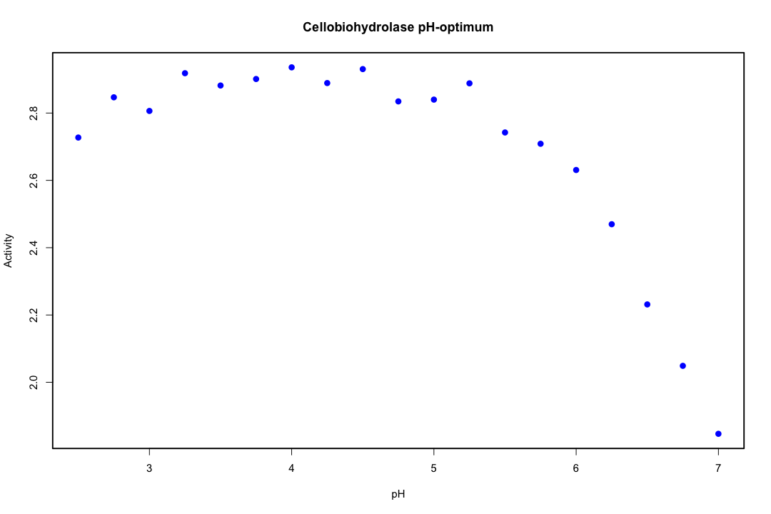
synthetic enzyme activity data

Now let's fit a 5-degree raw polynomial to this dataset:

raw.fit <- lm(y ~ poly(x, degree=5, raw=T), data)
print(summary(raw.fit))

which gives us the following result (I dropped the formula and residuals output):

Coefficients:
                                Estimate Std. Error t value Pr(>|t|)
(Intercept)                    1.834e+00  8.351e+00   0.220    0.830
poly(x, degree = 5, raw = T)1  7.837e-01  9.816e+00   0.080    0.938
poly(x, degree = 5, raw = T)2 -2.709e-01  4.477e+00  -0.061    0.953
poly(x, degree = 5, raw = T)3  5.261e-02  9.916e-01   0.053    0.958
poly(x, degree = 5, raw = T)4 -4.110e-03  1.069e-01  -0.038    0.970
poly(x, degree = 5, raw = T)5 -3.145e-05  4.496e-03  -0.007    0.995

Residual standard error: 0.05243 on 13 degrees of freedom
Multiple R-squared:  0.984,     Adjusted R-squared:  0.9779 
F-statistic: 160.1 on 5 and 13 DF,  p-value: 3.34e-11

What we get is a seemingly excellent fit (high $R^2$, significant F-stats etc.), but none of the coefficients seem to be significantly different from zero. If you try higher degrees [an exercise left to the reader], eventually the whole estimation breaks down, with NaN estimates. This is your punishment for using highly correlated predictors ($x, x^2, x^3, \ldots$) that make the columns of your design matrix almost linearly dependent, and the whole problem ill-conditioned.

Now let's perform the same estimation with orthogonal polynomials:

orth.fit <- lm(y ~ poly(x, degree=5, raw=F), data)
print(summary(orth.fit))

which gives us

Coefficients:
                                Estimate Std. Error t value Pr(>|t|)    
(Intercept)                    2.6758702  0.0120294 222.445  < 2e-16 ***
poly(x, degree = 5, raw = F)1 -1.0769949  0.0524348 -20.540 2.71e-11 ***
poly(x, degree = 5, raw = F)2 -0.9789274  0.0524348 -18.669 9.04e-11 ***
poly(x, degree = 5, raw = F)3 -0.2836844  0.0524348  -5.410 0.000119 ***
poly(x, degree = 5, raw = F)4 -0.0491978  0.0524348  -0.938 0.365213    
poly(x, degree = 5, raw = F)5 -0.0003668  0.0524348  -0.007 0.994525    
---
Signif. codes:  0 ‘***’ 0.001 ‘**’ 0.01 ‘*’ 0.05 ‘.’ 0.1 ‘ ’ 1

Residual standard error: 0.05243 on 13 degrees of freedom
Multiple R-squared:  0.984,     Adjusted R-squared:  0.9779 
F-statistic: 160.1 on 5 and 13 DF,  p-value: 3.34e-11

Points to note:

  1. The residual standard error, the $R^2$ values, the F-stats are exactly the same as before. We are essentially "fitting the same thing"...
  2. ...but differently. Look at the coefficients! The first 3 are now "significant", the rest aren't. So: what is the maximal degree of the polynomials to be used here? [Hint: 3 :-) ]

If you run the estimation with the 3-degree polynomials, you are in for another pleasant surprise:

orth.fit.3 <- lm(y ~ poly(x, degree=3, raw=F), data)
print(summary(orth.fit.3))

Check the coefficients in particular:

                              Estimate Std. Error t value Pr(>|t|)    
(Intercept)                    2.67587    0.01157 231.242  < 2e-16 ***
poly(x, degree = 3, raw = F)1 -1.07699    0.05044 -21.352 1.22e-12 ***
poly(x, degree = 3, raw = F)2 -0.97893    0.05044 -19.408 4.88e-12 ***
poly(x, degree = 3, raw = F)3 -0.28368    0.05044  -5.624 4.84e-05 ***

and you'll see that they are (practically) the same as in the degree=5 case. Which is neat, because you can build an empirical model now very easily: just run an orthogonal polynomial estimation, and keep the coefficients up to the highest that is still "significant".

As regards the model quality:

Residual standard error: 0.05044 on 15 degrees of freedom
Multiple R-squared:  0.9829,    Adjusted R-squared:  0.9795 
F-statistic: 288.1 on 3 and 15 DF,  p-value: 1.768e-13

These numbers differ slightly from the degree=5 case because the degrees of freedom is higher (15 vs 13).

Now you have your 3-degree polynomial empirical model and you can predict enzyme activity as a function of the pH to your heart's content.

Long story short: you are almost always better off by fitting orthogonal polynomials because the procedure is numerically better-conditioned. Should you ever need the raw polynomial coefficients, they can be calculated back from the orthogonal coefficients.

$\endgroup$

Your Answer

By clicking “Post Your Answer”, you agree to our terms of service and acknowledge you have read our privacy policy.

Not the answer you're looking for? Browse other questions tagged or ask your own question.