Quantile regression revealing different relationships at different quantiles: how?

Question

Quantile regression (QR) is sometimes said to reveal different relationships between variables at different quantiles of the distribution. E.g. Le Cook et al. "Thinking beyond the mean: a practical guide for using quantile regression methods for health services research" imply that QR allows for relationships between the outcomes of interest and the explanatory variables to be nonconstant across different values of the variables.

However, as far as I know, in a standard linear regression model $$ y = \beta_0 + \beta X + \varepsilon $$ with $\varepsilon$ being i.i.d. and independent of $X$, the QR estimator for the slope $\beta$ is consistent for the population slope (which is unique and does not anyhow vary across quantiles). That is, the object being estimated is always the same, regardless of the quantile. Admittedly, this is not the case for the intercept, since the QR intercept estimator aims at estimating a particular quantile of the error distribution. Taken together, I do not see how the different relationships between variables are supposed to be revealed at different quantiles via the QR. I guess this is a property of the standard linear regression model rather than a mistake in my understanding, but I am not sure.

I suppose the situation is different when some of the assumptions of the standard linear model are violated, e.g. under certain forms of conditional heteroskedasticity. Then perhaps the QR slope estimators converge to something else than the true slope of the linear model and somehow reveal different relationships at different quantiles.

What am I getting wrong? How should I properly understand/interpret the claim that quantile regression reveals different relationships between variables at different quantiles?

Answer 1

The "true slope" in a normal linear model tells you how much the mean response changes thanks to a one point increase in $x$. By assuming normality and equal variance, all quantiles of the conditional distribution of the response move in line with that. Sometimes, these assumptions are very unrealistic: variance or skewness of the conditional distribution depend on $x$ and thus, its quantiles move at their own speed when increasing $x$. In QR you will immediately see this from very different slope estimates. Since OLS only cares about the mean (i.e. the average quantile), you can't model each quantile separately. There, you are fully relying on the assumption of fixed shape of the conditional distribution when making statements on its quantiles.

EDIT: Embed comment and illustrate

If you are willing to make that strong assumtions, there is not much point in running QR as you can always calculate conditional quantiles via conditional mean and fixed variance. The "true" slopes of all quantiles will be equal to the true slope of the mean. In a specific sample, of course there will be some random variation. Or you might even detect that your strict assumptions were wrong...

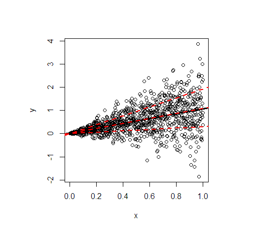
Let me illustrate by an example in R. It shows the least squares line (black) and then in red the modelled 20%, 50%, and 80% quantiles of data simulated according to the following linear relationship $$ y = x + x \varepsilon, \quad \varepsilon \sim N(0, 1) \ \text{iid}, $$ so that not only the conditional mean of $y$ depends on $x$ but also the variance.

• The regression lines of the mean and the median are essentially identical because of the symmetrical conditional distribution. Their slope is 1.
• The regression line of the 80% quantile is much steeper (slope 1.9), while the regression line of the 20% quantile is almost constant (slope 0.3). This suits well to the extremely unequal variance.
• Approximately 60% of all values are within the outer red lines. They form a simple, pointwise 60% forecast interval at each value of $x$.

The code to generate the picture:

library(quantreg)

set.seed(3249)
n <- 1000
x <- seq(0, 1, length.out = n)
y <- rnorm(n, mean = x, sd = x)

plot(y~x)

(fit_lm <- lm(y~x)) # intercept: 0.02445, slope: 1.04858 
abline(fit_lm, lwd = 3)

# quantile cuts
taus <- c(0.2, 0.5, 0.8)

(fit_rq <- rq(y~x, tau = taus))
#               tau= 0.2      tau= 0.5    tau= 0.8
# (Intercept) 0.00108228 -0.0005110046 0.001089583
# x           0.29960652  1.0954521888 1.918622442

lapply(seq_along(taus), function(i) abline(coef(fit_rq)[, i], lwd = 2, lty = 2, col = "red"))