I'm attending a econometric course and I'm new to time series analysis. They gave me a time series to analyze and I'm trying to apply all the things I learnt (and understood) to an actual time series.
The time series is about the Harmonised Index of Consumer Prices in Austria from Janaury 2000 to September 2017, with base=100 2015 get it from Eurostat.
I provide the dataset so you can reply it:
x<-ts(c(74.28,74.85,74.92,74.78,74.71,75.00,74.78,74.85,75.14,75.35,75.64,75.93,75.96,76.21,76.33,76.71,76.86,76.96,76.85,76.66,76.95,77.10,77.07,77.27,77.40,77.53,77.63,77.98,78.12,78.11,77.98,78.19,78.19,78.36,78.36,78.57,78.71,78.85,79.06,78.98,78.88,78.89,78.79,79.01,79.22,79.20,79.40,79.62,79.67,80.02,80.34,80.24,80.53,80.68,80.44,80.75,80.68,81.06,81.22,81.62,81.60,81.87,82.26,82.08,82.09,82.30,82.13,82.26,82.73,82.77,82.63,82.87,82.84,83.12,83.34,83.82,83.83,83.84,83.71,83.97,83.85,83.80,83.91,84.22,84.28,84.54,84.94,85.30,85.45,85.45,85.39,85.42,85.63,86.20,86.61,87.14,86.89,87.16,87.95,88.18,88.66,88.90,88.64,88.48,88.82,88.79,88.56,88.42,87.90,88.33,88.49,88.65,88.71,88.62,88.26,88.62,88.80,88.90,89.08,89.35,88.98,89.16,90.09,90.28,90.23,90.22,89.76,90.00,90.35,90.68,90.68,91.30,91.24,91.97,93.09,93.64,93.56,93.53,93.19,93.34,93.90,94.11,94.17,94.40,93.88,94.38,95.55,95.82,95.63,95.62,95.13,95.47,96.55,96.85,96.92,97.15,96.54,96.87,97.80,97.82,97.94,97.77,97.15,97.37,98.31,98.30,98.33,99.08,98.01,98.30,99.22,99.35,99.44,99.43,98.77,98.79,99.69,99.70,99.84,99.88,98.48,98.75,100.15,100.28,100.45,100.40,99.89,99.73,100.25,100.35,100.32,100.95,99.85,99.76,100.82,100.93,101.04,101.04,100.49,100.33,101.33,101.72,101.79,102.55,101.91,102.13,102.94,103.27,103.21,103.06,102.47,102.46,103.93),frequency = 12)
Usually I use Gretl, but in this case I'm gonna use R cause I found easier to explain the code.
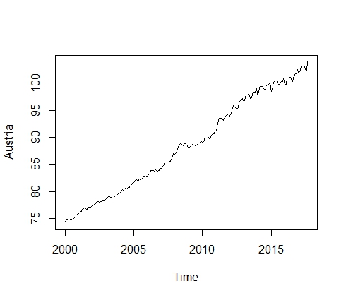
I follow the Box and Jenkins procedure. The first things I do is to visualize the time series. In this case, it's:
Firstly I wonder if there any kind of outliers (for example Addivite, Level shift, Innovation Outliers of Temporary change), that's not the case, I suppose. Obsviously it's not mean stationary and I have some doubts on the variance of the series. So I'm gonna consider a log-transformation and a difference of order 1.
d_log_x<-diff(log(x))
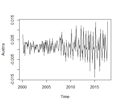
Now I have the time series with no trend. Now I should see the error part and the seasonality. The latter shows that seasonaliry increases during time:
At this point I remember that if the case that seasonality is evolutive, we prefer to consider a multiplicative model for time series. Anyway I'm gonna check now the periodgram of this series and that's what I get: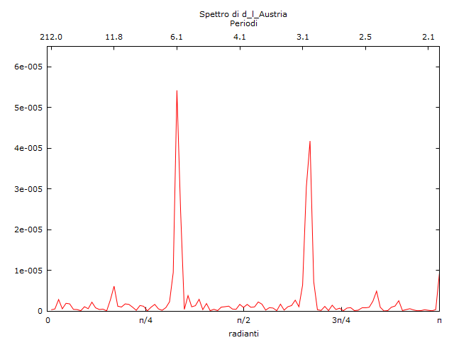
This should show me (if I'm not wrong) that we have a seasonaly every 6 months and 3 months.
Now I think of using a season differences, but which? I behave as follows: I see the standard deviations of the series with seasonal differences and I choose the lowest:
dif<-as.vector(c())
for(i in 1:48){dif<-rbind(dif, sd(diff(d_log_x,lag=i)))}
head(order(dif))
 [1] 12 36 24 48  6 18
So seasonal difference with order 12 gaves me the lowest sd.
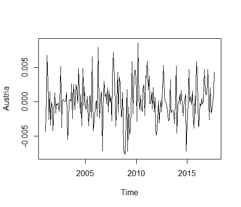
sddlog<-diff(d_log_x, lag=12)
plot(sddlog)
Now I can use acf and pacf to detect the best model, here they are:
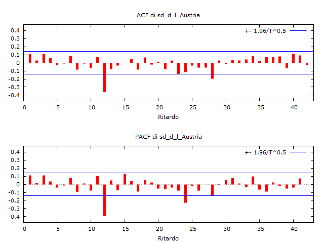
Now my question are:
- I don't know how to interpret it. I mean I would say that's only a seasonal arma ( but didn't I erase it?) and acf and pacf are so similar. I see both of them (seasonally speaking) with significant value at 12 lag and 24th lag (acf is not significant but almost it is) and then everything disappears. I would say it's a ARIMA(0,0)(0,1), but the PACF should not die so brutally, it should go to zero slowly.
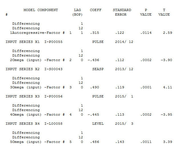
- Maybe should I use another kind of filter to eliminate the seasonality?
- Is it proper, maybe, to use a dummy variable?

