If z is uniform normal is $f(z;\theta)$ a normal distribution

Question

I am trying to understand the description of variational auto-encoders here

to quote the excerpt:

Before we can say that our model is representative of our dataset, we need to make sure that for every datapoint $X$ in the dataset, there is one (or many) settings of the latent variables which causes the model to generate something very similar to $X$. Formally, say we have a vector of latent variables $z$ in a high-dimensional space $Z$ which we can easily sample according to some probability density function (PDF) $P(z)$ defined over $Z$. Then, say we have a family of deterministic functions $f(z; θ)$, parameterized by a vector $θ$ in some space $Θ$, where $f : Z × Θ → X$ . $f$ is deterministic, but if $z$ is random and $θ$ is fixed, then $f(z; θ)$ is a random variable in the space $X$ . We wish to optimize $θ$ such that we can sample $z$ from $P(z)$ and, with high probability, $f(z; θ)$ will be like the $X$’s in our dataset. To make this notion precise mathematically, we are aiming maximize the probability of each $X$ in the training set under the entire generative process, according to: $$P(X) = \int_z P(X|z; θ)P(z)dz. \tag1$$ Here, $f(z; θ)$ has been replaced by a distribution $P(X|z; θ)$, which allows us to make the dependence of $X$ on $z$ explicit by using the law of total probability. The intuition behind this framework—called “maximum likelihood”— is that if the model is likely to produce training set samples, then it is also likely to produce similar samples, and unlikely to produce dissimilar ones. In VAEs, the choice of this output distribution is often Gaussian, i.e., $P(X|z; θ) = N (X| f(z; θ), σ 2 ∗ I)$. That is, it has mean $f(z; θ)$ and covariance equal to the identity matrix $I$ times some scalar $σ$ (which is a hyperparameter).

It would occur to me that if we are making a choice on any distribution it is on $z$. How can $P(X|z; θ)$ be chosen to be normal? and what is it with mean $f(z; θ)$? I am looking forward to understand the emboldened text and a little elucidation on what is being said in those lines

Answer 1

Ok, I had to ponder this for ages. Since when I first looked, I sort of came to the same conclusions as yourself :) So, I first wrote:

I'm not sure I entirely agree that 'the choice of this output distribution is often Gaussian', though it can be: I think we generally will have some kind of highly non-linear neural network, eg to take some latent values in z, and transform them into image of the digits 0,1,2, ... ; or some other images, etc.

And I concur with you: in a VAE, we are putting a prior on $z$, and sampling $z$, typically from an axis-aligned Gaussian, based on the output of the input, encoder, network.

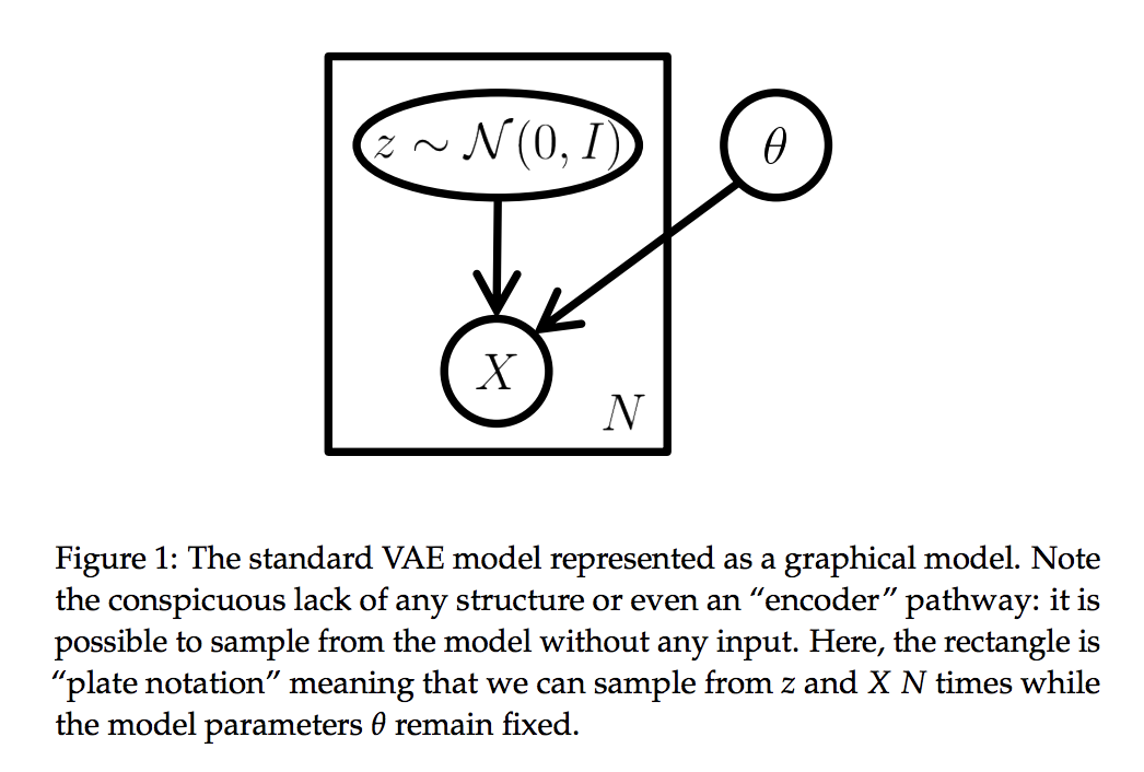
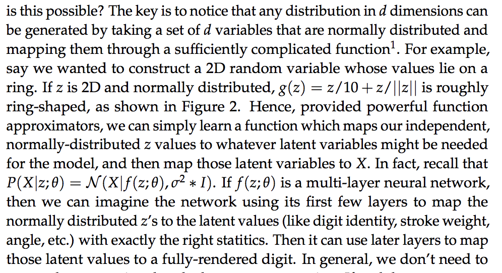
However, looking at the tutorial you linked, the text you have quoted is from the section '1.1 Preliminaries: latent variable models', and describes the graphical model shown in figure 1:

Later on, in section '2. Variational Autoencoders', it relates this model to the VAE model that we are typically used to seeing, with the input encoder neural net, followed by axis-aligned $z$-sampling, followed by a deterministic neural network, that reconstructs $X$. ie this bit:

... but, having written all this, I still couldn't quite see the answer to your question, i.e. why/how is $P(X \mid z)$ stochastic, and what does it mean?

Since normally in a VAE we essentially have the following layers, if we write it as a net:

• input inference network, models $q(z \mid X)$. Might have a bunch of layers, like convolutions or whatever. deterministic, given the weights, and the inputs
• then we take the outputs of the inference layer and transform them linearly into the mean and variance of an axis-aligned Gaussian. this bit is still deterministic
• we sample from this. stochastic and we use the reparameterization trick, so we can backprop through this
• at this point we have: $z$
• then we pass $z$ through the generation network, which is 100% entirely deterministic, though is probably another deep neural net, with deconvolution layers and so on
• the output of this network is then $X$

So, ... where is the stochastic bit of the generation network?

I think that the answer is hinted at by the likelihood expression written at the bottom of page 10:

$$ \def\Exp{\mathbb{E}} \Exp_{z \sim Q}[\log P(X \mid z)] $$

I think the point is that, whilst the $X$ is generated deterministically from $z$ in our network, but the error/loss term is calculated on the basis that these $X$ outputs are normally distributed, so that the loss is not almost surely zero. Otherwise if the outputs are not assumed to be normally distributed, and have a Dirac delta distribution, the probability of our output $X$ given our input $X$ is almost surely $0$.

There's a little bit of discussion in 2.4.3 'VAEs and the reparameterization parameter', that makes this clearer I think? They point out the effect of modifying the $\sigma$ in the Gaussian $P(X \mid z) \sim \mathcal{N}(f(z), \sigma^2 I)$, ie that as $\sigma \rightarrow 0$, then the output distribution tends to Dirac delta, and the likelihood of our reconstructed $X$ tends to $0$.

Edit: You ask:

The encoder gives us mean and std of the latent variables and we are forcing them to be a unit normal. So eventually, the encoder should only give us a zero and a one for all images ?

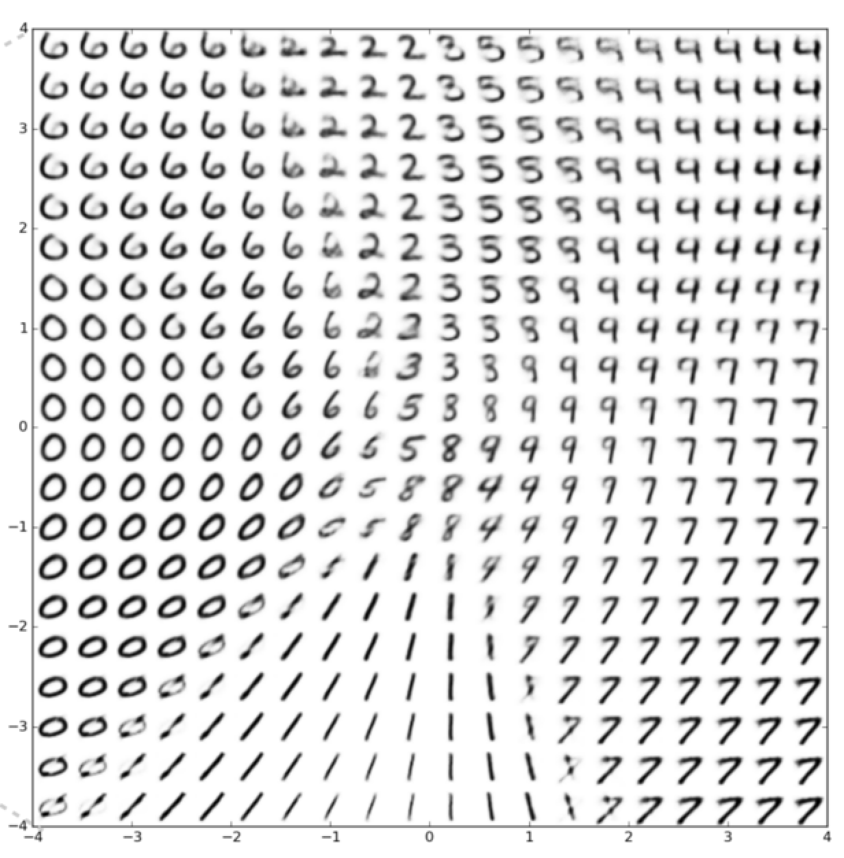
The z values will form a continuum around the origin, out to a radius of ~3 or so, at which radius the density of the Gaussians will be very tiny. The model will learn to place inputs that are similar to each other into nearby positions in the latent space. The z values will be reals, not binary 0/1, but eg maybe images of cars will end up near [0.3, 0.2] (if z is 2-dimensional), and maybe ostriches would be near [0.7, -0.3], and so on. The exact layout would depend on the distribution of the input data, and is learned in an entirely unsupervised manner. There are some great images around on the web, for example at http://blog.fastforwardlabs.com/2016/08/12/introducing-variational-autoencoders-in-prose-and.html :

This is showing how images learned from mnist look at different positions in the 2-dimensional z space that a model has learned.

You ask:

how can we expect the decoder to generate the exact image in the input when we randomly sample from a normal distribution?

So, the idea is that points in the latent space which are nearby should be similar. So, by encoding to a particular part of the latent space, the generator will generator an image similar-ish (but not identical) to the input. We want it to sample so that it can adequately explore the latent space, make the meaning of adjacent points in the latent space similar-ish to each other. Otherwise we might as well just throw the data into a lookup table :)

On the output, the Gaussian blurs somewhat the output images, but it's not like the latent space cannot influence the generated image at all. The extent to which the output is blurred is controlled by the $\sigma$ hyperparameter. Too large, and the output will be very blurry. Too small and learning will be slow.

Edit 2: You ask:

can you dumb this down for me a little - "I think the point is that, whilst the XX is generated deterministically from zz in our network, but the error/loss term is calculated on the basis that these XX outputs are normally distributed, so that the loss is not almost surely zero. Otherwise if the outputs are not assumed to be normally distributed, and have a Dirac delta distribution, the probability of our output XX given our input XX is almost surely 0." the loss is Variational lower bound + L2 norm between generated and input images?

whilst we can think of what we are calculating as a loss, and it works as a loss, what we are actually calculating is a probability distribution over output images, and the likelihood of our original image, given that probability distribution. It may or may not end up as an expression similar or identical to MSE loss, but the actual underlying approach is different.

MSE Loss:

• difference between target and output
• square it
• take the mean across all the elements in the vector (if there's more than one)

In our case, we have a probability distribution for $X$ given $z$:

$$ p(X \mid z) $$

and its a Gaussian:

$$ p(X \mid z) = \mathcal{N}(X; \cdot, \cdot) $$

The variance of the Gaussian is fixed, to be $\sigma^2$, a hyperparameter:

$$ p(X \mid z) = \mathcal{N}(X; \cdot, \sigma^2) $$

The mean of the Gaussian is the output of our decoder neural net:

$$ p(X \mid z) = \mathcal{N}(X; f(z, \theta), \sigma^2) $$

Then, we take our input image, and we calculate the likelihood, based on this Gaussian, by simply plugging in the numbers:

$$ p(X \mid z) = \mathcal{N}(\text{input image}; \text{neural net output}, \text{hyperparameter}) $$

Answer 2

You ask:

How can $P(X|z;θ)$ be chosen to be normal? and what is it with mean $f(z;θ)$?

For the first question, I think we can answer this question by asking:

Why we make an autoencoder variational in the first place?

It is explained in this post that we do this because we want to make an autoencoder generative. By using a classical autoencoder the latent distribution is discrete. So when the decoder samples from a gap between clusters in the latent space, it will have no idea how to deal with it. So, instead of a deterministic mapping $f(z; \theta)$, we want to add some noise to it. So we can write $f(z; \theta) + \epsilon$, and this $\epsilon$ can be sampled from a normal distribution, and that's why $P(x|z)$ can be chosen to be normal.

Of course, there are other choices of this $P(x|z)$, as is pointed out in this paper on page 11, $P(x|z)$ can also be chosen to be a multivariate Bernoulli.

For the second question:

$f(z; \theta)$ is only a mapping. Say the latent space is $p$ dimensional, and the data space is $d$ dimensional, then this $f(z;\theta)$ will just eat a $p$ dimensional vector and returns a $d$ dimensional vector. But note that this mapping can be non-linear since we are using a neural network to implement this, which is unlike what we have in factor analysis, in which the mapping is linear.