Why does minimizing the MAE lead to forecasting the median and not the mean?

Question

From the Forecasting: Principles and Practice textbook by Rob J Hyndman and George Athanasopoulos, specifically the section on accuracy measurement:

A forecast method that minimizes the MAE will lead to forecasts of the median, while minimizing the RMSE will lead to forecasts of the mean

Can someone give an intuitive explanation of why minimizing the MAE leads to the forecasting the median and not the mean? And what does this means in practice?

I have asked a customer: "what is more important for you to make mean forecasts more accurate or to avoid very inaccurate forecasts?". He said that to made mean forecasts more accurate have higher priority. So, in this case, should I use MAE or RMSE? Before I read this citation I believed that MAE will be better for such condition. And now I doubt.

Answer 1

It's useful to take a step back and forget about the forecasting aspect for a minute. Let's consider just any distribution $F$ and assume we wish to summarize it using a single number.

You learn very early in your statistics classes that using the expectation of $F$ as a single number summary will minimize the expected squared error.

The question now is: why does using the median of $F$ minimize the expected absolute error?

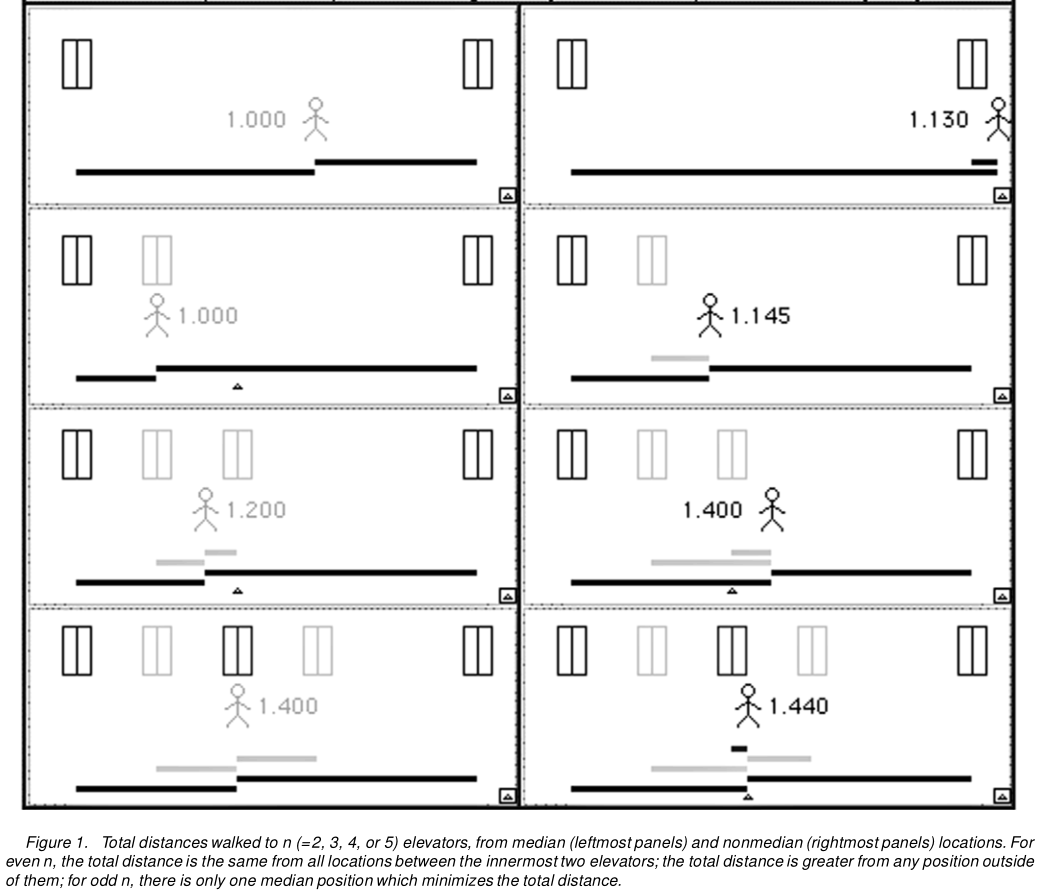
For this, I often recommend "Visualizing the Median as the Minimum-Deviation Location" by Hanley et al. (2001, The American Statistician). They did set up a little applet along with their paper, which unfortunately probably doesn't work with modern browsers any more, but we can follow the logic in the paper.

Suppose you stand in front of a bank of elevators. They may be arranged equally spaced, or some distances between elevator doors may be larger than others (e.g., some elevators may be out of order). In front of which elevator should you stand to have the minimal expected walk when one of the elevators does arrive? Note that this expected walk plays the role of the expected absolute error!

Suppose you have three elevators A, B and C.

• If you wait in front of A, you may need to walk from A to B (if B arrives), or from A to C (if C arrives) - passing B!
• If you wait in front of B, you need to walk from B to A (if A arrives) or from B to C (if C arrives).
• If you wait in front of C, you need to walk from C to A (if A arrives) - passing B - or from C to B (if B arrives).

Note that from the first and last waiting position, there is a distance - AB in the first, BC in the last position - that you need to walk in multiple cases of elevators arriving. Therefore, your best bet is to stand right in front of the middle elevator - regardless of how the three elevators are arranged.

Here is Figure 1 from Hanley et al.:

This generalizes easily to more than three elevators. Or to elevators with different chances of arriving first. Or indeed to countably infinitely many elevators. So we can apply this logic to all discrete distributions and then pass to the limit to arrive at continuous distributions.

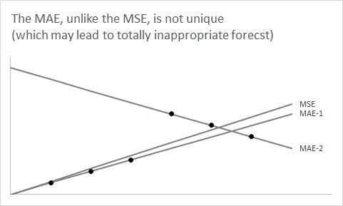
To double back to forecasting, you need to consider that underlying your point forecast for a particular future time bucket, there is a (usually implicit) density forecast or predictive distribution, which we summarize using a single number point forecast. The above argument shows why the median of your predictive density $\hat{F}$ is the point forecast that minimizes the expected absolute error or MAE. (To be more precise, any median may do, since it may not be uniquely defined - in the elevator example, this corresponds to having an even number of elevators.)

And of course the median may be quite different than the expectation if $\hat{F}$ is asymmetric. One important example is with low-volume count-data, especially intermittent-time-series. Indeed, if you have a 50% or higher chance of zero sales, e.g., if sales are Poisson distributed with parameter $\lambda\leq \ln 2$, then you will minimize your expected absolute error by forecasting a flat zero - which is rather unintuitive, even for highly intermittent time series. I wrote a little paper on this (Kolassa, 2016, International Journal of Forecasting).

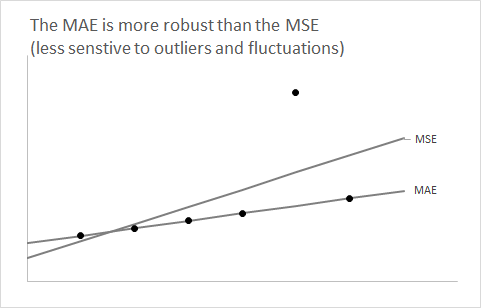
Thus, if you suspect that your predictive distribution is (or should be) asymmetric, as in the two cases above, then if you wish to get unbiased expectation forecasts, use the rmse. If the distribution can be assumed symmetric (typically for high-volume series), then the median and the mean coincide, and using the mae will also guide you to unbiased forecasts - and the MAE is easier to understand.

Similarly, minimizing the mape can lead to biased forecasts, even for symmetric distributions. This earlier answer of mine contains a simulated example with an asymmetrically distributed strictly positive (lognormally distributed) series can meaningfully be point forecasted using three different point forecasts, depending on whether we want to minimize the MSE, the MAE or the MAPE.

Answer 2

Stephan's answer gives you an intuitive explanation of why minimizing the absolute average error gives you the median. To answer which of the MSE, MAE or MAPE you should minimize:

• The MAE is robust, meaning it is less sensitive to outliers. Imagine a series of $n$ points with an error a million times greater that what it should be. The MSE will pull the forecast a million / $n$ times, while the MAE will only be pulled by 1 unit (fig. 1).

• Unfortunately, minimizing the MAE can lead to multiple solutions (fig. 2).

So my recommendation is:

1. Fit a model using the MSE.
2. Start an MAE-based regression with the fitted parameters.
3. Compare both forecasts. If they are very different, your data may have anomalies.

Fig. 1:

Fig. 2:

Answer 3

All the aforementioned explanations are great, just suggesting a shorter one.

Assuming you would use some value which isn't the median to minimize MAE then there are A examples above the value and B examples below it such that w.l.o.g $A>B$. Then by increasing the value by $\epsilon>0$ the error reduces by $\epsilon$ for all $A$ examples and increases by $\epsilon$ for all $B$ examples, so overall the error was reduced by $(A-B)\epsilon>0$.

This is true for any value where $A \neq B$, I.e. any value but the median.