Is this linear model overfitting when I add more parameters?

Question

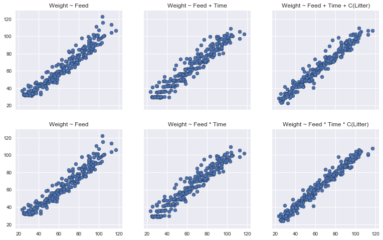
I am trying to figure out if my models are overfitting. This is a trend I noticed with my actual dataset associating metadata with compositional data.

The more parameters I add, the better the model's performance. When I do interactions with the multiplication operator the mean-square-error decreases and the likelihood increases.

Amy overfitting? Should this be expected? If I was overfitting would I see a drop in likelihood?

# Import packages
import statsmodels.api as sm
import statsmodels.formula.api as smf
import matplotlib.pyplot as plt
import numpy as np

# Get data
data = sm.datasets.get_rdataset('dietox', 'geepack').data
# Remove nulls
data = data.dropna(how="any", axis=0)
# Training data
idx_training = np.random.RandomState(0).choice(data.shape[0], size=int(data.shape[0]*0.7), replace=False)
idx_testing = list(set(range(data.shape[0])) - set(idx_tr))

X_training = data.iloc[idx_training,:]
X_testing = data.iloc[idx_testing,:]

# Preview
print(data.head())
print()
#      Weight       Feed  Time   Pig  Evit  Cu  Litter
# 1  27.59999   5.200005     2  4601     1   1       1
# 2  36.50000  17.600000     3  4601     1   1       1
# 3  40.29999  28.500000     4  4601     1   1       1
# 4  49.09998  45.200001     5  4601     1   1       1
# 5  55.39999  56.900002     6  4601     1   1       1

# Run models
y = "Weight"
attributes = ["Feed", "Time", "C(Litter)"]

fig, ax = plt.subplots(ncols=3, nrows=2, figsize=(13,8), sharex=True, sharey=True)
for i, operator in enumerate(["+", "*"]):
    print(f"Operator --> {operator}", "==============", sep="\n")
    for j in range(len(attributes)):
        # Build model
        query_attrs = attributes[:j+1]
        formula = y + " ~ " + f" {operator} ".join(query_attrs)
        model_results = smf.mixedlm(formula, X_training, groups=X_training["Pig"]).fit()
        # Get data
        y_true = X_testing[y]
        y_hat = model_results.predict(X_testing)
        # Performance
        likelihood = model_results.llf
        mse = np.power(model_results.resid,2).mean()
        rho = stats.pearsonr(y_true.values, y_hat.values)[0]
        print(formula, len(formula)*"-", f"\tLog-likelihood\t{likelihood}", f"\tMean-Squared-Error\t{mse}", f"\tPearson's rho\t{rho}", sep="\n")
        print()
        # Plot
        ax[i,j].scatter(y_true, y_hat, edgecolor="black")
        ax[i,j].set_title(formula)

     Weight       Feed  Time   Pig  Evit  Cu  Litter
1  27.59999   5.200005     2  4601     1   1       1
2  36.50000  17.600000     3  4601     1   1       1
3  40.29999  28.500000     4  4601     1   1       1
4  49.09998  45.200001     5  4601     1   1       1
5  55.39999  56.900002     6  4601     1   1       1

Operator --> +
==============
Weight ~ Feed
-------------
    Log-likelihood  -1610.8433385451501
    Mean-Squared-Error  12.581854321567183
    Pearson's rho   0.9647573890325062

Weight ~ Feed + Time
--------------------
    Log-likelihood  -1475.0535695263359
    Mean-Squared-Error  6.708542197869
    Pearson's rho   0.958639465612475

Weight ~ Feed + Time + C(Litter)
--------------------------------
    Log-likelihood  -1417.3142217330767
    Mean-Squared-Error  6.6968475983201925
    Pearson's rho   0.975122313069836

Operator --> *
==============
Weight ~ Feed
-------------
    Log-likelihood  -1610.8433385451501
    Mean-Squared-Error  12.581854321567183
    Pearson's rho   0.9647573890325062

Weight ~ Feed * Time
--------------------
    Log-likelihood  -1475.456924646852
    Mean-Squared-Error  6.619270700334347
    Pearson's rho   0.9614174630247257

Weight ~ Feed * Time * C(Litter)
--------------------------------
    Log-likelihood  -1405.2281927890776
    Mean-Squared-Error  3.670974515594324
    Pearson's rho   0.9822717811213982

Answer 1

But the VIF may be high because of high multicollinearity.

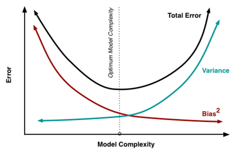
Usually, increasing the complexity of model will decrease the bias but will increase the variance. Conversely, decreasing the complexity of model will increase the bias but will reduce the variance. In both the cases the error will go up. Basic thing to do in such scenario is to balance between both. Please refer to this graph for more understanding

I would suggest you to use Lasso regression, which will reduce the coefficient term of each attribute such that significant attributes will have comparatively higher coefficient while the insignificant attributes will have negligible coefficient, diminishing the effect of insignificant/correlated attributes.

Answer 2

Generally, overfitted model works well with the training data but does not reflect well with the test data, which in turn leads to high RMSE value. What I would suggest is that, run the same model for multiple sets of samples (80% of the data for training purpose and 20% of the data for training purpose), calculate the RMSE value with its corresponding test data. If the average of all RMSE scores are closer to one, then the model is just right. If the average of all RMSE scores are on the higher side, then the model is overfitted!

For example

1. We have 10000 rows of data points with 5 features (4 independent and 1 dependent variable)

2. Choose 80% of 10000 as training data, which is 8000 data points at random and build the model

3. Use this model to predict test data, remaining 20% of 10000, which is 2000

4. Calculate RMSE for the current test set

5. Repeat step 2 to 4 multiple times, say 100 times, and calculate the RMSE values for all the 100 samples

6. If the average RMSE value of these 100 samples are closer to zero then your model is a good fit, if this value is much bigger, then the model is not a good fit and the model should be revisited

Hope I have answered your question!