Is the best model always one with best test score, even though it looks overfit?

Question

I'm making a binary classification model using gradient boosting (lightgbm). I usually use learning curves to check if my model is overfitting. The metric I'm using is sklearn's average precision-recall score.

When use the default model parameters parameters, I get a test metric of 0.69 but when I look at the learning curve there is a large difference between the train and validation scores with iteration number (as shown in first image).

Usually, when this happens, I would reduce model complexity. In this case I reduced max_depth, num_leaves and max_bin. The learning curve is shown below, but its test score is 0.63.

My question is, which is the better model. The one with best test score that looks overfit or the one with similar learning curves?

Answer 1

One recommendation: look at the distribution of your scores and add confidence intervals to your curves. This may help to contextualize whether the 0.69 score you're getting in model A test is really higher from the 0.63 model B test score. If there's enough variation in your scores, this difference may not be meaningful.

Otherwise, you could argue that model A is a bit more performant than model B, BUT, you could also argue that model A is less adept at pinpointing the "true" patterns in your data. In other words, model B is probably better at explaining what's going on, whereas model A has probably picked up on a lot of patterns/noise that you don't care about.

Having said that, it somewhat depends on what your goals. Are you in a situation where it's a priority to have a model that is closer to understanding what's going on your idea, even if it takes a small hit in performance? Or is eking out performance the priority, even if your model has misinterpreted the signal? I think most people would go with a model that has a better idea of what it's doing, ie model B, but there are some circles where performance is everything (not weighing on whether this is valid) and model A would be chosen. Just be aware, model A is something of a wild card - you don't know what patterns it has latched on to, and it's not unreasonable to say that model A could perform a lot worse in the real world relative to model B.

Answer 2

params = {}
params['learning_rate'] = 0.2
params['boosting_type'] = 'goss'
params['objective'] = 'multiclassova'
params['metric'] = ['multi_error', 'multi_logloss']
params['sub_feature'] = 0.8
params['num_leaves'] = 15
params['min_data'] = 600
params['tree_learner'] = 'voting'
params['bagging_freq'] = 3
params['num_class'] = 3
params['max_depth'] = -1
params['max_bin'] = 512
params['verbose'] = -1
params['is_unbalance'] = True
#params['lambda_l2'] = 60

aa = lgb.train(params,
               d_train,
               init_model = aa,
               valid_sets=[d_train, d_test],
               evals_result=evals_result,
               num_boost_round=3000,
               early_stopping_rounds = 2000,   
               feature_name=f_names,
               verbose_eval=10,
               categorical_feature=f_names)

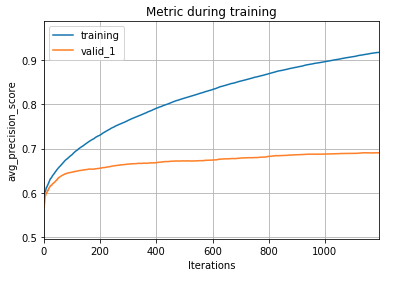
Here above is an example from my codes. By feeding verbose_eval = 10, you will be able to print the loss metric of both the training and the test sets at every 10 iterations. You will see the point where your test loss does not decrease anymore, and afterwhile it increases, starting to overfit. Do not compare two with their loss numerically, they can differ. Moreover, by early_stopping_rounds you can make your algorithm automatically stop at a point where your loss stops decreasing. Moreover, you can plot the training and test losses that evals_result has recorded for you per iteration to see how your test losses behave in time:

lgb.plot_metric(evals_result, metric='multi_error')
plt.show()

lgb.plot_metric(evals_result, metric='multi_logloss')
plt.show()

Note: LightGBM allows us to use more than one metric, it is usually wise to monitor multiple rather than observing one. For example, multi_logloss can still keep decreasing, where multi_error starts to increase, from experience.