My question is a follow-up to this question, following through on @Isabelle Ghement's excellent series of responses. I just want to run this past some people in the know to see if what I am doing is correct.
I am conducting a longitudinal logistic regression testing blinding in a clinical trial. I want to know whether actual treatment allocation (placebo vs active) predicts odds of guessing that one had been allocated to active treatment at each of four time points, 4, 8, 12, and 24 weeks after the start of the trial. Basically I am testing the blind at each of four time points during the trial.
Apparently in order to estimate the general effects of certain predictor variables in mixed-effects models with nonlinear link functions you need to estimate marginal coefficients (otherwise you get subject-specific effects). You can do this using the GLMMadaptive package.
First I ran the model. It is a random intercepts model testing the effects of two fixed factors, group (actual treatment allocation, two level factor with two levels Placebo vs Active), week (time marker, four levels, week4, week8, week12, and week24) and their interaction on log-odds of guessing active treatment (outcome variable guess, where 1 is guessing active treatment and 0 is guessing placebo).
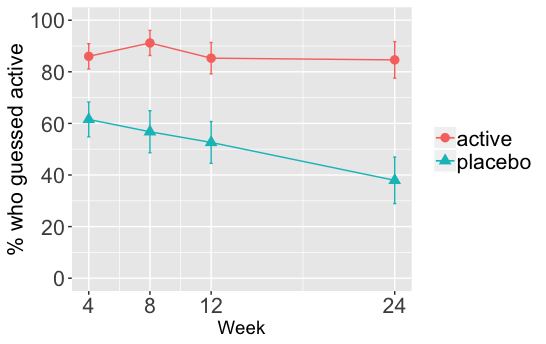
As a guide, this is the graph of the proportion who guessed active over the four time points
The model looks like this
glmmAdapt <- mixed_model(fixed = guess ~ group * week,
                         random = ~ 1 | id,
                         data = df,
                         family = binomial())
...and this is the command to obtain marginal coefficients, as well as the output
margMod <- marginal_coefs(glmmAdapt, std_errors = T)

#                               Estimate Std.Err z-value   p-value
# (Intercept)                     0.5390  0.2796  1.9281 0.0538445
# groupActive                     1.2602  0.4806  2.6223 0.0087348
# weekweek08                     -0.2044  0.2574 -0.7938 0.4273142
# weekweek12                     -0.4543  0.2608 -1.7418 0.0815422
# weekweek24                     -0.8936  0.3361 -2.6590 0.0078378
# groupActive:weekweek08          0.8840  0.6077  1.4548 0.1457201
# groupActive:weekweek12          0.2173  0.5097  0.4263 0.6698632
# groupActive:weekweek24          1.2141  0.6078  1.9977 0.0457512
Now, what I want to do is to test simple effects of treatment group on guessed treatment at each of the four timepoints.
The group comparison at the first time point, week 4, is easy: its coefficient and p-value, 1.26 and 0.4806 respectively, can be taken straight from the output above. Although the z-value (2.622) and p-value (0.0087) are supplied, we can calculate them from the coefficient (1.2602) and standard error (0.4806) for the comparison
# z-value
(z4 <- 1.2602/0.4806)
[1] 2.622139

# p-value
(p4 <- pnorm(z4, 0, 1, lower.tail = F)*2)
[1] 0.008737979
Calculating the simple effects of group at the other three time points, however, is not so easy. You can obtain the coefficient for each comparison easily enough. I will perform the test for between-group difference in log-odds of guessing active at week 8, but the same principle will apply to the same test at week 12 and at week 24. We get the coefficient for the week 8 comparison by adding together the groupActive coefficient (beta 2) and the groupActive:weekweek08 coefficient (beta 6).
# coefficient for between-group difference at week 8
(coef8 <- 1.2602 + 0.8840)
[1] 2.1442
The hard part is calculating the standard error for the comparison. Following @Isabelle Ghement's instructions, based on this post, we can obtain the standard error for the comparison via the formula
$se(beta 2 + beta 6)^2 = var(beta 2) + var(beta 6) + 2cov(beta 2, beta 6)$
We obtain the variance and covariances from the variance-covariance table supplied by the marg_coefs() function
margMod$var_betas

#                      (Intercept) groupActive weekweek08 weekweek12 weekweek24 groupActive:weekweek08 groupActive:weekweek12 groupActive:weekweek24
# (Intercept)               0.0782     -0.0830    -0.0326    -0.0222    -0.0324                 0.0196                 0.0270                 0.0164
# groupActive              -0.0830      0.2310     0.0267     0.0101     0.0161                -0.0656                -0.0978                -0.0599
# weekweek08               -0.0326      0.0267     0.0663     0.0301     0.0326                -0.0622                -0.0245                -0.0061
# weekweek12               -0.0222      0.0101     0.0301     0.0680     0.0343                -0.0422                -0.0814                -0.0323
# weekweek24               -0.0324      0.0161     0.0326     0.0343     0.1129                -0.0326                -0.0414                -0.1053
# groupActive:weekweek08    0.0196     -0.0656    -0.0622    -0.0422    -0.0326                 0.3692                 0.0914                 0.1487
# groupActive:weekweek12    0.0270     -0.0978    -0.0245    -0.0814    -0.0414                 0.0914                 0.2598                 0.0867
# groupActive:weekweek24    0.0164     -0.0599    -0.0061    -0.0323    -0.1053                 0.1487                 0.0867                 0.3694
Now, based on this table, the variance for $beta 2$ (groupActive coefficient) is 0.2310 and the variance for $beta 6$ (groupActive:weekweek08 coefficient) is 0.3692.
The covariance for $(beta 2, beta 6)$ is -0.0656. So the full formula for the standard error of the comparison is
(seB2B6 <- sqrt(0.2310 + 0.3692 + 2*-0.0656))
[1] 0.6848357
We get the test statistic, the z-value, for the comparison by dividing the coefficient for the comparison by its standard error
# z-value
(zB2B6 <- 2.1442/0.6848357)
[1] 3.13097
And finally we get the p-value via
# p-value
pnorm(3.13097, 0, 1, lower.tail = F)*2
[1] 0.0017423
My question is Did I follow the steps for obtaining the p-value correctly?

