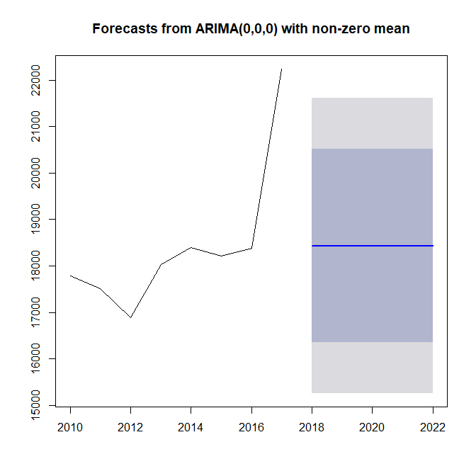
auto.arima() fits an ARIMA(0,0,0) model with a nonzero mean to your data. This means that it believes your data are independent and identically normally distributed. The optimal forecast for such a series is the expectation. Since your data are assumed to be identically distributed, this mean is identical for all future time periods. Thus the flat line.
This is not only an effect of little data, but also of the fact that any dynamics like trend are not obvious at all. Any trend would be solely driven by the last observation.
Note the large prediction intervals, which are due to the large noise in your data.

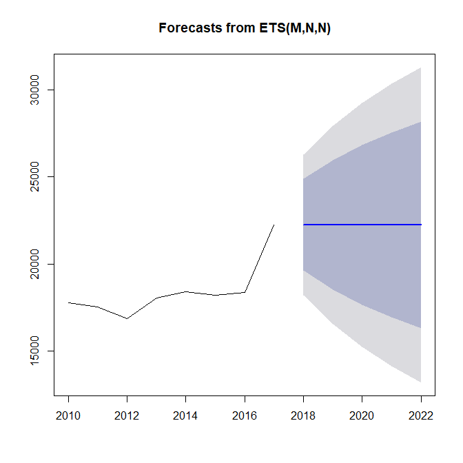
Here is what an ETS model fits, which is essentially exponential smoothing. It also does not fit a trend, but it adapts more quickly to what it believes to be a changing level. Note that the fitted multiplicative errors lead to widening prediction intervals.

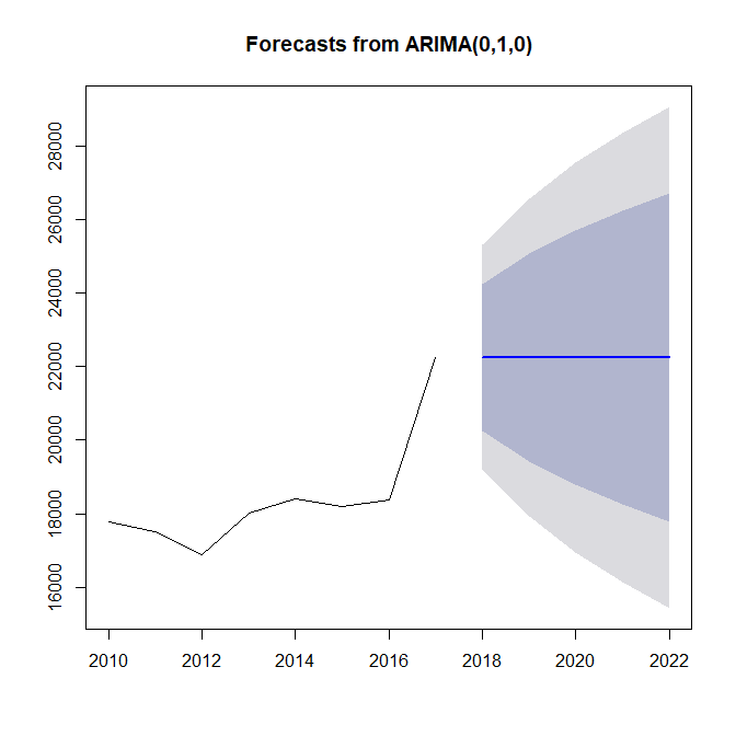
If you believe that your last observation represents a new level on which your time series will stay for the future, you could go with this model. Alternatively, you could fit an ARIMA($p$,1,$q$) model, i.e., allow auto.arima() to fit any ARMA($p$,$q$) model to successive differences or increments. If so, you get an ARIMA(0,1,0) model, i.e., auto.arima() believes that increments are iid. Note that there is no "non-zero mean", i.e., the increments are assumed to be distributed with a zero mean. In other words: the forecast will start off your last observation, but predict no change.

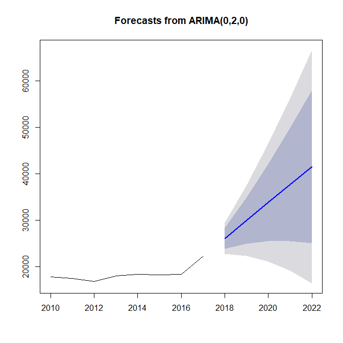
Finally, if you believe that there truly is a trend in your data, you can fit an ARIMA($p$,2,$q$) model to your data, i.e., an ARMA model fitted to second differences. You get this:

This can go badly wrong, especially if you forecast out for five years and make any far-reaching decisions based on this forecast.
I personally don't think the initial ARIMA(0,0,0) forecast with a nonzero mean "makes no sense". It's exactly what I would expect from auto.arima(), which is an automatic piece of software designed to give reasonable forecasts over a wide range of situations.
In your case, an automatic forecasting algorithm may not be what you need at all, particularly if you have only a single series to forecast. The most interesting data point in your history is the last, and how you interpret it will determine what forecast you believe "makes sense". So the first order of business would be to understand what happened here. Did anything change in 2017 compared to previous years? Was a substitute product discontinued? Were marketing efforts increased? In each case, will the situation that led to this data point persist in the future, or be even stronger? The answers to questions like these will guide you to a more reasonable forecast.
In the meantime, I recommend the excellent free online book Forecasting: Principles and Practice (2nd ed.) by Athanasopoulos & Hyndman.
R code:
library(forecast)
euro <- ts(c(17785,17515,16880,18036,18400,18211,18382,22248),start=2010)
plot(forecast(auto.arima(euro),h=5))
plot(forecast(ets(euro),h=5))
plot(forecast(auto.arima(euro,d=1),h=5))
plot(forecast(auto.arima(euro,d=2),h=5))

