Can I interpret the inclusion of a quadratic term in logistic regression as indicating a turning point?

Question

In a Logistic Regression with linear and quadratic terms only, if I have a linear coefficient $\beta_1$ and quadratic coefficient $\beta_2$, can I say that that there is turning point of the probability at $-\beta_1 / (2\beta_2)$?

Answer 1

Yes, you can.

---

The model is

$$\Pr(Y=1) = \frac{1}{1+ \exp(-[\beta_0 + \beta_1 x + \beta_2 x^2])}.$$

When $\beta_2$ is nonzero, this has a global extremum at $x = -\beta_1 / (2\beta_2)$.

Logistic regression estimates these coefficients as $(b_0, b_1, b_2)$. Because this is a maximum likelihood estimate (and ML estimates of functions of parameters are the same functions of the estimates) we can estimate the location of the extremum is at $-b_1/(2b_2)$.

A confidence interval for that estimate would be of interest. For datasets that are large enough for the asymptotic maximum likelihood theory to apply, we can find the endpoints of this interval by re-expressing $\beta_0 + \beta_1 x + \beta_2 x^2$ in the form

$$\beta_0 + \beta_1 x + \beta_2 x^2 = \beta_0 - \beta_1^2/(4\beta_2) + \beta_2(x + \beta_1/(2\beta_2))^2 = \beta + \beta_2(x + \gamma)^2$$

and finding how much $\gamma$ can be varied before the log likelihood decreases too much. "Too much" is, asymptotically, one-half the $1-\alpha/2$ quantile of a chi-squared distribution with one degree of freedom.

This approach will work well provided the ranges of $x$ cover both sides of the peak and there are a sufficient number of $0$ and $1$ responses among the $y$ values to delineate that peak. Otherwise, the location of the peak will be highly uncertain and the asymptotic estimates may be unreliable.

---

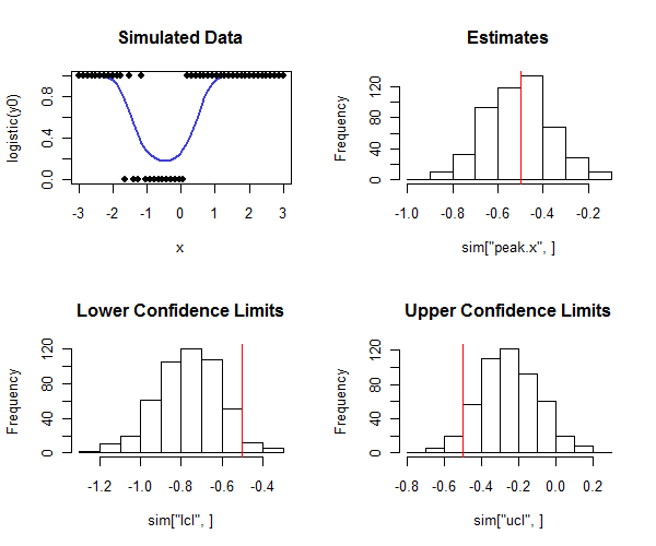
R code to carry this out is below. It can be used in a simulation to check that the coverage of the confidence intervals is close to the intended coverage. Notice how the true peak is $-1/2$ and--by looking at the bottom row of histograms--how most of the lower confidence limits are less than the true value and most of the upper confidence limits are greater than the true value, as we would hope. In this example the intended coverage was $1 - 2(0.05) = 0.90$ and the actual coverage (discounting four out of $500$ cases where the logistic regression did not converge) was $0.91$, indicating the method is working well (for the kinds of data simulated here).

n <- 50            # Number of observations in each trial
beta <- c(-1,2,2)  # Coefficients
x <- seq(from=-3, to=3, length.out=n)
y0 <- cbind(rep(1,length(x)), x, x^2) %*% beta

# Conduct a simulation.
set.seed(17)
sim <- replicate(500, peak(x, rbinom(length(x), 1, logistic(y0)), alpha=0.05))

# Post-process the results to check the actual coverage.
tp <- -beta[2] / (2 * beta[3])
covers <- sim["lcl",] <= tp & tp <= sim["ucl",]
mean(covers, na.rm=TRUE) # Should be close to 1 - 2*alpha

# Plot the distributions of the results.
par(mfrow=c(2,2))
plot(x, logistic(y0), type="l", lwd=2, col="#4040d0", main="Simulated Data",ylim=c(0,1))
points(x, rbinom(length(x), 1, logistic(y0)), pch=19)
hist(sim["peak.x",], main="Estimates"); abline(v=tp, col="Red")
hist(sim["lcl",], main="Lower Confidence Limits"); abline(v=tp, col="Red")
hist(sim["ucl",], main="Upper Confidence Limits"); abline(v=tp, col="Red")

logistic <- function(x) 1 / (1 + exp(-x))

peak <- function(x, y, alpha=0.05) {
  #
  # Estimate the peak of a quadratic logistic fit of y to x
  # and a 1-alpha confidence interval for that peak.
  #
  logL <- function(b) {
    # Log likelihood.
    p <- sapply(cbind(rep(1, length(x)), x, x*x) %*% b, logistic)
    sum(log(p[y==1])) + sum(log(1-p[y==0]))
  }
  f <- function(gamma) {
    # Deviance as a function of offset from the peak.
    b0 <- c(b[1] - b[2]^2/(4*b[3]) + b[3]*gamma^2, -2*b[3]*gamma, b[3])
    -2.0 * logL(b0)
  }
  # Estimation.
  fit <- glm(y ~ x + I(x*x), family=binomial(link = "logit"))
  if (!fit$converged) return(rep(NA,3))

  b <- coef(fit)
  tp <- -b[2] / (2 * b[3])

  # Two-sided confidence interval:
  # Search for where the deviance is at a threshold determined by alpha.
  delta <- qchisq(1-alpha, df=1)
  u <- sd(x)
  while(fit$deviance - f(tp+u) + delta > 0) u <- 2*u # Find an upper bound
  l <- sd(x)
  while(fit$deviance - f(tp-l) + delta > 0) l <- 2*l # Find a lower bound
  upper <- uniroot(function(gamma) fit$deviance - f(gamma) + delta, 
                   interval=c(tp, tp+u))
  lower <- uniroot(function(gamma) fit$deviance - f(gamma) + delta, 
                   interval=c(tp-l, tp))

  # Return a vector of the estimate, lower limit, and upper limit.
  c(peak=tp, lcl=lower$root, ucl=upper$root)
}