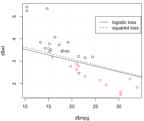
It seems like you've fixed the issue in your particular example but I think it's still worth a more careful study of the difference between least squares and maximum likelihood logistic regression.
Let's get some notation. Let $L_S(y_i, \hat y_i) = \frac 12(y_i - \hat y_i)^2$ and $L_L(y_i, \hat y_i) = y_i \log \hat y_i + (1 - y_i) \log(1 - \hat y_i)$. If we're doing maximum likelihood (or minimum negative log likelihood as I'm doing here), we have
$$
\hat \beta_L := \text{argmin}_{b \in \mathbb R^p} -\sum_{i=1}^n y_i \log g^{-1}(x_i^T b) + (1-y_i)\log(1 - g^{-1}(x_i^T b))
$$
with $g$ being our link function.
Alternatively we have
$$
\hat \beta_S := \text{argmin}_{b \in \mathbb R^p} \frac 12 \sum_{i=1}^n (y_i - g^{-1}(x_i^T b))^2
$$
as the least squares solution. Thus $\hat \beta_S$ minimizes $L_S$ and similarly for $L_L$.
Let $f_S$ and $f_L$ be the objective functions corresponding to minimizing $L_S$ and $L_L$ respectively as is done for $\hat \beta_S$ and $\hat \beta_L$. Finally, let $h = g^{-1}$ so $\hat y_i = h(x_i^T b)$. Note that if we're using the canonical link we've got
$$
h(z) = \frac{1}{1+e^{-z}} \implies h'(z) = h(z) (1 - h(z)).
$$
For regular logistic regression we have
$$
\frac{\partial f_L}{\partial b_j} = -\sum_{i=1}^n h'(x_i^T b)x_{ij} \left( \frac{y_i}{h(x_i^T b)} - \frac{1-y_i}{1 - h(x_i^T b)}\right).
$$
Using $h' = h \cdot (1 - h)$ we can simplify this to
$$
\frac{\partial f_L}{\partial b_j} = -\sum_{i=1}^n x_{ij} \left( y_i(1 - \hat y_i) - (1-y_i)\hat y_i\right) = -\sum_{i=1}^n x_{ij}(y_i - \hat y_i)
$$
so
$$
\nabla f_L(b) = -X^T (Y - \hat Y).
$$
Next let's do second derivatives. The Hessian
$$H_L:=
\frac{\partial^2 f_L}{\partial b_j \partial b_k} = \sum_{i=1}^n x_{ij} x_{ik} \hat y_i (1 - \hat y_i).
$$
This means that $H_L = X^T A X$ where $A = \text{diag} \left(\hat Y (1 -
\hat Y)\right)$. $H_L$ does depend on the current fitted values $\hat Y$ but $Y$ has dropped out, and $H_L$ is PSD. Thus our optimization problem is convex in $b$.
Let's compare this to least squares.
$$
\frac{\partial f_S}{\partial b_j} = - \sum_{i=1}^n (y_i - \hat y_i) h'(x^T_i b)x_{ij}.
$$
This means we have
$$
\nabla f_S(b) = -X^T A (Y - \hat Y).
$$
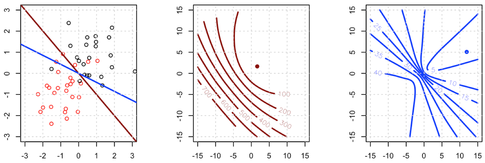
This is a vital point: the gradient is almost the same except for all $i$ $\hat y_i (1 - \hat y_i) \in (0,1)$ so basically we're flattening the gradient relative to $\nabla f_L$. This'll make convergence slower.
For the Hessian we can first write
$$
\frac{\partial f_S}{\partial b_j} = - \sum_{i=1}^n x_{ij}(y_i - \hat y_i) \hat y_i (1 - \hat y_i) = - \sum_{i=1}^n x_{ij}\left( y_i \hat y_i -
(1+y_i)\hat y_i^2 + \hat y_i^3\right).
$$
This leads us to
$$
H_S:=\frac{\partial^2 f_S}{\partial b_j \partial b_k} = - \sum_{i=1}^n x_{ij} x_{ik} h'(x_i^T b) \left( y_i - 2(1+y_i)\hat y_i + 3 \hat y_i^2 \right).
$$
Let $B = \text{diag} \left( y_i - 2(1+y_i)\hat y_i + 3 \hat y_i ^2 \right)$. We now have
$$
H_S = -X^T A B X.
$$
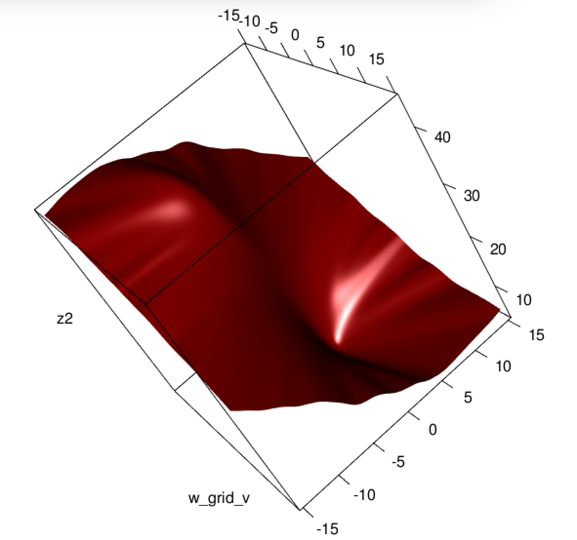
Unfortunately for us, the weights in $B$ are not guaranteed to be non-negative: if $y_i = 0$ then $y_i - 2(1+y_i)\hat y_i + 3 \hat y_i ^2 = \hat y_i (3 \hat y_i - 2)$ which is positive iff $\hat y_i > \frac 23$. Similarly, if $y_i = 1$ then $y_i - 2(1+y_i)\hat y_i + 3 \hat y_i ^2 = 1-4 \hat y_i + 3 \hat y_i^2$ which is positive when $\hat y_i < \frac 13$ (it's also positive for $\hat y_i > 1$ but that's not possible). This means that $H_S$ is not necessarily PSD, so not only are we squashing our gradients which will make learning harder, but we've also messed up the convexity of our problem.
All in all, it's no surprise that least squares logistic regression struggles sometimes, and in your example you've got enough fitted values close to $0$ or $1$ so that $\hat y_i (1 - \hat y_i)$ can be pretty small and thus the gradient is quite flattened.
Connecting this to neural networks, even though this is but a humble logistic regression I think with squared loss you're experiencing something like what Goodfellow, Bengio, and Courville are referring to in their Deep Learning book when they write the following:
One recurring theme throughout neural network design is that the gradient of the cost function must be large and predictable enough to serve as a good guide for the learning algorithm. Functions that saturate (become very flat) undermine this objective because they make the gradient become very small. In many cases this happens because the activation functions used to produce the output of the hidden units or the output units saturate. The negative log-likelihood helps to avoid this problem for many models. Many output units involve an exp function that can saturate when its argument is very negative. The log function in the negative log-likelihood cost function undoes the exp of some output units. We will discuss the interaction between the cost function and the choice of output unit in Sec. 6.2.2.
and, in 6.2.2,
Unfortunately, mean squared error and mean absolute error often lead to poor results when used with gradient-based optimization. Some output units that saturate produce very small gradients when combined with these cost functions. This is one reason that the cross-entropy cost function is more popular than mean squared error or mean absolute error, even when it is not necessary to estimate an entire distribution $p(y|x)$.
(both excerpts are from chapter 6).
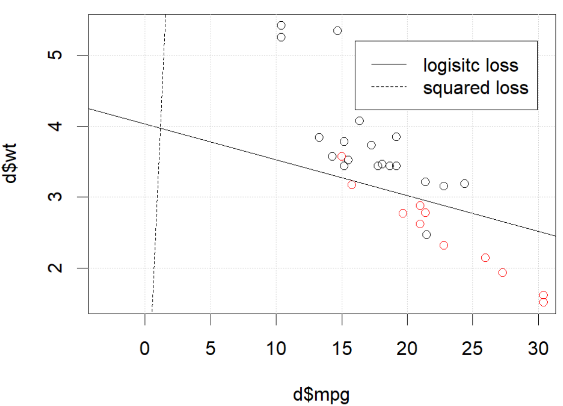
 What is happening here? The optimization does not converge? Logistic loss is easier to optimize comparing to squared loss? Any help would be appreciated.


optimtells you it hasn't finished, that's all: it is converging. You might learn a great deal by rerunning your code with the additional argumentcontrol=list(maxit=10000), plotting its fit, and comparing its coefficients to the original ones. $\endgroup$