2
$\begingroup$

I have a time series of data points, and I know that they have a double-exponential probability density function:

$P(t) = A_1 \exp(-t/\tau_1) + A_2 \exp(-t/\tau_2)$

where $\tau_1 < \tau_2$.

I would like to know an efficient and accurate way to estimate the probability distribution parameters ($A_1, A_2, \tau_1, \tau_2)$. By efficient, I mean requiring fewer data points to attain an accurate estimate.

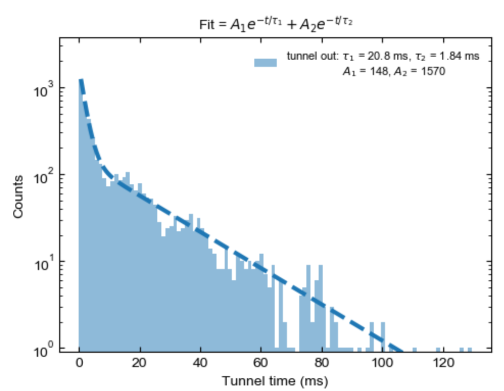
My current approach consists of binning the data and applying fitting the double exponential, as shown below. While this approach works, it requires a lot of data points for an accurate estimate. Are there any better methods to extract the probability distribution parameters?

Sample dataset

The sample data file is uploaded at http://s000.tinyupload.com/?file_id=49278196312362946370

This is an example dataset of time-series data, which are labelled as tunnel times. My current solution is to bin the data, followed by fitting. I should emphasize that I am looking for a better approach.

Double exponential fit Note that in this image, $A_1$ and $A_2$ are not normalized

$\endgroup$
12
  • $\begingroup$ Do you mean "efficient" in terms of using the information in the data (so as to better estimate the parameters) or do you mean "computationally fast"? $\endgroup$
    – Glen_b
    Commented Jul 26, 2019 at 3:13
  • $\begingroup$ Good point! I mean requiring fewer data points for an accurate estimate. I'll update the post accordingly. And what do you mean by specifying a model? Are you referring to the double exponential probability distribution? $\endgroup$ Commented Jul 26, 2019 at 5:17
  • $\begingroup$ The plot appears to have a "Y" axis of counts, and not probability. To my eye the plot does not appear to use binned data. My apology, but I am having difficulty relating the question to the plot. $\endgroup$ Commented Jul 27, 2019 at 1:36
  • $\begingroup$ @JamesPhillips I have slightly modified the figure to clarify that it actually is binned data. Each bin corresponds to there being X occurrences within a time interval. $\endgroup$ Commented Jul 28, 2019 at 23:52
  • $\begingroup$ @Glen_b I'm not sure I'm following your reasoning. I could very well know that the data points follow a certain probability distribution. Perhaps a point of confusion is that I may have erroneously used the term "probability distribution" while I meant "probability density function (PDF)". $\endgroup$ Commented Jul 28, 2019 at 23:56

1 Answer 1

1
$\begingroup$

If what you want is to estimate the parameters of a mixture of two exponential distributions given your data, then I would recommend using a maximum likelihood approach but only if your data collection method meets certain assumptions.

Your description uses the term "time series data" but you're completely ignoring anything dealing with time order. So if there is some serial correlation over time, then you don't have a random sample of independent observations which is required for the maximum likelihood procedure given below.

And if you do have a random sample from a mixture of two exponential distributions, then you certainly don't want to perform a regression on the binned counts (other than for maybe obtaining starting values for the parameters).

Here's the R code to find the maximum likelihood estimates:

# Get data and change to milliseconds
tt = read.table("tunnel_times.txt", header=FALSE, col.names="t")
tt$t = 1000*tt$t

# Define log of the likelihood
logL = function(p, t) {
  a1 = p[1]
  tau1 = p[2]
  tau2 = p[3]
  sum(log((a1/tau1)/exp(t/tau1) + ((1 - a1)/tau2)/exp(t/tau2)))
}

# Set starting values for the parameters
a10 =0.5
tau10 = 2
tau20 = 20

# Find maximum likelihood estimates and estimated standard errors
sol = optim(c(a10, tau10, tau20), logL, t=tt$t, control=list(fnscale=-1),
  lower=c(0,0,0), upper=c(1,Inf,Inf), method="L-BFGS-B", hessian=TRUE)

# Show maximum likelihood estimates
a1 = sol$par[1]
tau1 = sol$par[2]
tau2 = sol$par[3]
# Estimated standard errors
covmat = -solve(sol$hessian)
# Show summary of results
cat("   a1 =", a1, "se =", covmat[1,1]^0.5, "\n",
    "tau1 =", tau1, " se =", covmat[2,2]^0.5,  "\n",
    "tau2 =", tau2, " se =", covmat[3,3]^0.5,  "\n")

#   a1 = 0.4600806 se = 0.01219539 
# tau1 = 1.716867  se = 0.06293959 
# tau2 = 18.63834  se = 0.4648512 

Now show histogram and estimated density

hist(tt$t, freq=FALSE, breaks=100, las=1, main="Histogram and estimated density")
t = c(0:120)
lines(t, (a1/tau1)/exp(t/tau1) + ((1 - a1)/tau2)/exp(t/tau2), col="red", lwd=3)
box()
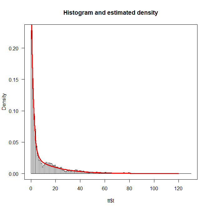
Histogram and estimated density

One of your questions is about how much data is needed for an "adequate" fit. You'll first need to define what you mean by adequate. That definition should not be "I'll know it when I see it." The definition depends on your needs and it likely a separate question as to how to characterize adequacy.

Alternatively, you can "punt" and just give the standard errors for the parameters and let someone else decide on adequacy. (That particular sentence is not meant to be sarcastic. Many of us simply provide estimates with measures of precision. The adequacy will depend on whoever uses the results and their standards can certainly and appropriately change over time. Or the results are meant to inform several different objectives and so there is no single definition of adequacy.)

$\endgroup$

Your Answer

By clicking “Post Your Answer”, you agree to our terms of service and acknowledge you have read our privacy policy.

Not the answer you're looking for? Browse other questions tagged or ask your own question.