PowerSim function (simr package) indicates 100% power for small sample dataset, regardless of effect size, alpha level, or if fixed/random slopes

Question

I am using the simr package to do power analyses for lmer multilevel models I have run, to determine the power of a pilot dataset for future research.

The dataset consists of 46 subjects with approximately 148 trials within subjects at level 1, and I've tried the power simulations at the original sample, at an extended sample of 800, with fixed slopes, random slopes, and at alpha of .001 and .05. The effect size from the original dataset was .10, but I have also expanded it to 1 and 4.

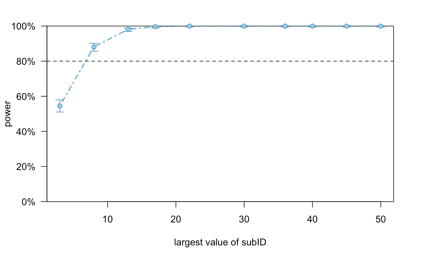
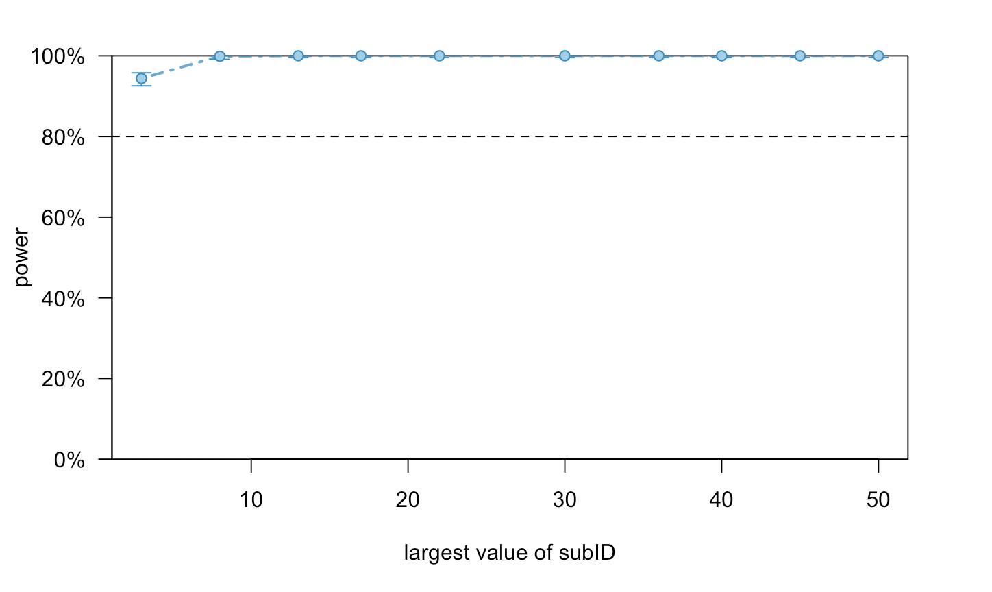
Reliably, I am getting a power of 100% for every variant of this simulation I've run. I did a power curve analysis and plotted it as well. It suggests that I have above 80% power by as low as 10 subjects for the random slopes model and as low as 2-3 subjects for the fixed slopes model. Frankly, this seems very odd to me and doesn't make much sense. The only post hoc justification I can make here is that my level 1 sample is decently large (148 per level 2 sample).

Primarily, I am confused how/why I am getting such high power and if it is because I executed something incorrectly or there is something off with my data or execution. If it is not something I did wrong, why would a sample of 2-3 subjects (with 148 trials within) at fixed slopes and 10 subjects at random slopes give you power of over 80%? That does not make sense to me and seems very off. It also seems off that I reliably get a power of 100% regardless of what parameters I change.

Any insights or thoughts would be great.

Further details are below...

Random slopes model appears as:

Linear mixed model fit by REML ['lmerMod']
Formula: selfRespT2 ~ feedback + selfRespT1 + valEstF + (feedback + selfRespT1 +      valEstF | subID)
   Data: fullDf1
Control: lmerControl(optimizer = "bobyqa", optCtrl = list(maxfun = 2e+05))

REML criterion at convergence: 21206.9

Scaled residuals: 
    Min      1Q  Median      3Q     Max 
-4.5158 -0.6078  0.0341  0.6287  3.6362 

Random effects:
 Groups   Name        Variance Std.Dev. Corr             
 subID    (Intercept) 1.450505 1.20437                   
          feedback    0.005708 0.07555  -0.55            
          selfRespT1  0.030467 0.17455  -0.78  0.15      
          valEstF     0.007138 0.08448  -0.73  0.53  0.19
 Residual             1.449100 1.20379                   
Number of obs: 6525, groups:  subID, 46

Fixed effects:
            Estimate Std. Error t value
(Intercept)  0.98865    0.20401   4.846
feedback     0.10127    0.01313   7.712
selfRespT1   0.51978    0.02795  18.599
valEstF      0.16395    0.02160   7.590

Correlation of Fixed Effects:
           (Intr) fedbck slfRT1
feedback   -0.458              
selfRespT1 -0.662  0.074       
valEstF    -0.698  0.268  0.016

Then simulation appears as:

sim2 <- powerSim(MLM.1.1, fixed("feedback", "z"), seed = 2, nsim = 800, alpha = .05)

Power for predictor 'feedback', (95% confidence interval):
      100.0% (99.54, 100.0)

Test: z-test
      Effect size for feedback is 0.10

Based on 800 simulations, (4 warnings, 0 errors)
alpha = 0.05, nrow = 6525

Time elapsed: 0 h 37 m 36 s

nb: result might be an observed power calculation

Fixed slopes model appears as:

Linear mixed model fit by REML ['lmerMod']
Formula: selfRespT2 ~ feedback + selfRespT1 + valEstF + (1 | subID)
   Data: fullDf1
Control: lmerControl(optimizer = "bobyqa", optCtrl = list(maxfun = 2e+05))

REML criterion at convergence: 21547.8

Scaled residuals: 
    Min      1Q  Median      3Q     Max 
-4.3314 -0.6033  0.0533  0.6255  3.6128 

Random effects:
 Groups   Name        Variance Std.Dev.
 subID    (Intercept) 0.1058   0.3252  
 Residual             1.5597   1.2489  
Number of obs: 6525, groups:  subID, 46

Fixed effects:
            Estimate Std. Error t value
(Intercept) 0.941441   0.107714    8.74
feedback    0.097369   0.007106   13.70
selfRespT1  0.516865   0.010486   49.29
valEstF     0.187282   0.018181   10.30

Correlation of Fixed Effects:
           (Intr) fedbck slfRT1
feedback   -0.179              
selfRespT1 -0.120 -0.207       
valEstF    -0.758 -0.006 -0.301

Simulation for fixed slopes model appears as:

sim4 <- powerSim(MLM.1.2, fixed("feedback", "z"), seed = 2, nsim = 800, alpha = .05)

Power for predictor 'feedback', (95% confidence interval):
      100.0% (99.54, 100.0)

Test: z-test
      Effect size for feedback is 0.10

Based on 800 simulations, (4 warnings, 0 errors)
alpha = 0.05, nrow = 6525

Time elapsed: 0 h 36 m 55 s

nb: result might be an observed power calculation

I receive the same 100% power when I manually change the effect size of .1 to 1 or to 4, as well as when I change the alpha to .001 instead of .05.

Power curve analysis for random slopes model appears as:

Power curve analysis for fixed slopes model appears as:

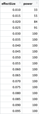
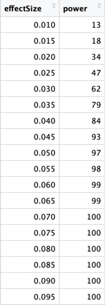
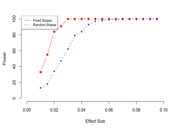
UPDATE: I manipulated the effect size and here too it rapidly gets to 100% power.

Fixed slopes, changing effect size

Random slopes, changing effect size

Visualized changing effect sizes:

Answer 1

The problem here might have been that you tried to calculate observed power. This always leads to misleading power estimates.

A high power basically just means that you were able to find a significant effect with your study design and data. If you base a power calculation on an observed significant effect, of course the power will be 100%. This is one of the reasons why observed power calculations are actually not very reasonable. What you could do is i.e. to take your observed effect and manipulate that in the sense of lowering the slope value to see if your study design would have been able to also detect a smaller effect. You could also take your observed effect and manipulate other factors such as sample size or model parameters, to see how power would change with sample size etc.

A larger effect size is easier to detect than a smaller one, so a change from .10 to 1 or 4 will not tell you anything new. Lower it instead of manipulating the effect to be even larger.