How to calculate the autocovariance of a time-series model when the expectation is taken over different lags?

Question

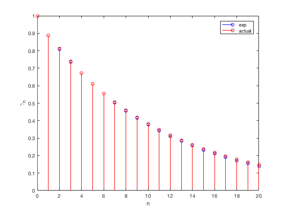
Let $ Z_t$ be a weakly stationary stochastic (WSS) process of order $p$ modeled as an autoregressive model.

$Z_t = \phi_{1} Z_{t-1} + \phi_{2} Z_{t-2} + \phi_{p} Z_{t-p} + a_t $ .

where $a_t$ is the random component.

One learns from most books on Time Series Analysis that to calculate the autcorrelation function of $Z_t$, one must multiply $Z_t$ by $Z_{t-j}$ and, after that, the expectation of the product should be calculated. The result would be:

$\mathbb{E}(Z_t.Z_{t-j}) = \phi_{1}.\mathbb{E}(Z_{t-1}.Z_{t-j}) + \phi_{2}.\mathbb{E}(Z_{t-2}.Z_{t-j}) + ... + \phi_{p}.\mathbb{E}(Z_{t-p}.Z_{t-j}) + \phi_{1}.\mathbb{E}(a_{t}.Z_{t-j}) $

Since $Z_{t-j}$ only correlates to the noise until $a_{t-j}$, $\mathbb{E}(a_{t}.Z_{t-j}) = 0, j > 0$, one could simply the equation above as the following:

$\gamma_j = \phi_1.\gamma_{j-1} + \phi_2.\gamma_{j-2} + ... + \phi_p.\gamma_{j-p}, j > 0$

where $\gamma_j$ is the covariance of $Z_t$ and $Z_{t-j}$.

Although this seems simple, I have been having trouble trying to show the result for a numerical example. For instance, let a known WSS autoregressive model $Y_t$be:

$Y_t = 0.8 Y_{t-1} + 0.6 Y_{t-2} + a_t $.

If $j = 1$, then $Y_{t-j}$ = $Y_{t-1} = 0.8 Y_{t-2} + 0.6 Y_{t-3} + a_{t-1} $.

If I multiply $Y_t$ by $Y_{t-1}$, and then take the expected value, I'd be calculating the covariance of $Y_t$ and its first lag, $Y_{t-1}$:

$\gamma_j = cov(Y_t,Y_{t-1})$

In my numerical example, that would be:

$\mathbb{E}(Y_t . Y_{t-1}) = 0.64 \mathbb{E}(Y_{t-1}.Y_{t-2}) + 0.48 \mathbb{E}(Y_{t-2}.Y_{t-2}) + 0.8 \mathbb{E}(Y_{t-2}.a_t) + 0.48\mathbb{E}(Y_{t-1}.Y_{t-3}) + 0.36\mathbb{E}(Y_{t-2}.Y_{t-3}) + 0.6 \mathbb{E}(Y_{t-3}.a_t) + 0.8\mathbb{E}(Z_{t-1}.a_{t-1}) + 0.6\mathbb{E}(Z_{t-2}.a_{t-1}) + \mathbb{E}(a_{t}.a_{t-1})$

Simplifying the equation above, one gets:

$\mathbb{E}(Y_t . Y_{t-1}) = 0.64 \mathbb{E}(Y_{t-1}.Y_{t-2}) + 0.48 \mathbb{E}(Y_{t-2}.Y_{t-2}) + 0.48\mathbb{E}(Y_{t-1}.Y_{t-3}) + 0.36\mathbb{E}(Y_{t-2}.Y_{t-3}) + 0.8\mathbb{E}(Z_{t-1}.a_{t-1})$

How do I proceed from here?

Knowing this is assumed to be a WSS process, I know that the covariance function relies upon only the lag $j$.

Can I then say that $\mathbb{E}(Y_{t-2}.Y_{t-3}) = \mathbb{E}(Y_{t-1}.Y_{t-2})$ since $2-3 = 1-2$?

I know that the correlation of $(Y_{t-2},Y_{t-2})$ would be one, but the covariance will not necessarily be.

---

Edit: As @gunes rightly pointed out, the correlation of $\mathbb{E}(Y_{t-1}.Y_{t-2})$ will not be one. What I should've written was that the correlation of $(Y_{t-2},Y_{t-2})$ will be one, but its covariance won't.

Answer 1

Yes, the following is correct due to WSS: $\mathbb{E}[Y_{t-2}Y_{t-3}]=\mathbb{E}[Y_{t-1}Y_{t-2}]$. By the way, the correlation of $Y_{t-1}$ and $Y_{t-2}$ is not $1$, and there is no such thing as the correlation of $\mathbb{E}[Y_{t-1}Y_{t-2}]$. For the solution, you'll find $\gamma_0,\gamma_1$ and then solve the difference equation you mentioned for $\gamma_n$ with these initial conditions. You also need to know $\sigma_a^2$.

The problem with your example is roots of the characteristic equation are not all outside the unit circle (if you use backshift operator), so the process cannot be both stationary and causal. So, let's try the following instead: $y_t=0.8y_{t-1}+0.1y_{t-2}+a_t$, and let $\sigma_a^2=1$.

$$\gamma_0=\operatorname{cov}(y_t,y_t)=0.65\gamma_0+1+0.16\gamma_1$$ $$\gamma_1=\operatorname{cov}(y_t,y_{t-1})=0.8\gamma_0+0.1\gamma_1$$ From these two equations we find that $\gamma_1=\frac{8}{9}\gamma_0,\gamma_0\approx 4.81$. For larger lags, we have the following difference equation: $$\gamma_n=0.8\gamma_{n-1}+0.1\gamma_{n-2}$$ which has solution of the form, where $r_i$ are the roots of $r^2-0.8r-0.1$: $$\gamma_n=ar_1^n+br_2^n$$ $a,b$ can be found via initial conditions, $\gamma_0,\gamma_1$ as $b\approx 0.0206\gamma_0$ and $a\approx0.9794\gamma_0$. Here is a Matlab code and experimental and theoretical autocorrelations (not covariance but we can scale out everything by $\gamma_0$):

clearvars
close all
clc

rng(42);

N = 1e5;
y = zeros(1,N);
y(1) = -.1;
y(2) = .2;

b = [0.8 0.1];
for i = 3:N
    y(i) = b(1)*y(i-1)+b(2)*y(i-2)+randn();
end

acorr = autocorr(y);

b = 0.0206; a = 0.9794;
r1 = 0.91; r2 = -0.11;

n = 0:length(acorr)-1;
acorr_h = r1.^n * a + r2.^n * b;

stem(n, acorr, 'b'); 
hold on;
stem(n, acorr_h, 'r');
xlabel('n'); ylabel('\gamma_n');
legend('exp', 'actual');