Chart indicates homoscedasticity but Breusch-Pagan test p<.001

Question

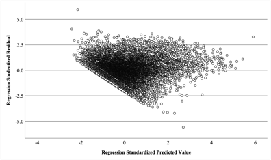
I am writing my master's thesis and doing multiple regression analysis for hypotheses testing. I transformed the data using ln and use a sample with N = 15,000. As a result of the assumption test, I got the following scatterplot.

The scatter plot with standardized residual against studentized value is typical for homoscedasticity of residuals which is a triangular shape.

However, a Breusch-Pagan test shows a significance of 0.000 and thus rejects the null hypothesis of homoscedasticity. According to the test, it is heteroscedastic.

Should I still assume homoscedasticity and therefore interpret the results using robust standard errors and the HC3 method? I am using SPSS.

Answer 1

It is likely that a Breusch-Pagan test shows such a level of statistical significance (i.e. p < .001) because you have a relatively large sample size (N = 15,000). Visual inspection does indeed show a triangular pattern, indicating potential heteroskedasticity. From my experience, I would be more inclined to use the visual interpretation as it is more telling

Edit and further Clarification

1. Given a relatively large sample size (N = 15,000) the Breusch-Pagan test may be sensitive to small deviations from homoscedasticity. This may explain p < .001 level of statistical significance

2. The triangular shape of the residuals indeed warrants to consider heteroskedasticity

Note: Credit for clarification goes to @SalMangiafico for his input

Answer 2

The fundamental identity

residual $\equiv$ observed $-$ fitted

implies that each distinct observed value defines a straight line with slope $-1$ in a plot of residual versus fitted and in particular that a sharp lower limit to observed values gives the lowest possible such line, i.e. a sharp diagonal bound to the configuration of data points in that plot. The use of studentized or standardized quantities complicates the algebra while the geometric essentials remain the same. This artefact has often been noticed on Cross Validated and is evident in the plot shown.

While it is reported that "the data" have been transformed using natural logarithms it remains unclear whether that refers to transformation of the response variable and/or to transformation of one or more predictors. Regardless of that, the plot to me suggests that multiple regression has been applied in a space where it may not be optimal.

It would be helpful to get clarification on the nature of the response variable and on its lower limit in principle and in practice. For example, if data concern counts and the minimum number of counts is 1 and the distribution of counts is highly skewed and/or relationships appear nonlinear, then the logarithm might well seem a helpful transformation. But then the logarithm must be 0 or more, which is itself unproblematic except that conditional distributions of residuals will struggle to be even symmetric, let alone normal. To the point, homoscedasticity is also likely to be impossible even as an ideal given other plausible behaviour.

In several other cases I have seen multiple regression has been applied to responses that cannot be negative, or that can only be positive. In this situation it is generally preferable to use a generalised linear model with logarithmic link, or Poisson regression in a suitably general interpretation of the latter. There is little point in expecting plain or vanilla regression assumptions (or, as some prefer to say, ideal conditions) to apply even roughly in spaces that make them impossible.