Does the multivariate Central Limit Theorem (CLT) hold when variables exhibit perfect contemporaneous dependence?

Question

The title sums up my question, but for clarity consider the following simple example. Let $X_i \overset{iid}{\backsim} \mathcal{N}(0, 1)$, $i = 1, ..., n$. Define: \begin{equation} S_n = \frac{1}{n} \sum_{i=1}^n X_i \end{equation} and \begin{equation} T_n = \frac{1}{n} \sum_{i=1}^n (X_i^2 - 1) \end{equation} My question: Even though $S_n$ and $T_n$ are perfectly dependent when $n = 1$, do $\sqrt{n} S_n$ and $\sqrt{n} T_n$ converge to a joint normal distribution as $n \rightarrow \infty$?

The motivation: My motivation for the question stems from the fact that it feels odd (but wonderful) that $S_n$ and $T_n$ are perfectly dependent when $n = 1$, yet the implication of the multivariate CLT is that they approach independence as $n \rightarrow \infty$ (this would follow since $S_n$ and $T_n$ are uncorrelated for all $n$, hence if they are asymptotically joint normal, then they must also be asymptotically independent).

Thanks in advance for any answers or comments!

ps, If you can provide any references etc then all the better!

Answer 1

The short answer as I understand your q is "yes, but ..." the rates of convergence on S, T, and any other moments are not necessarily the same -- check out determining bounds with the Berry-Esseen Theorem.

In case I misunderstand your q, Sn and Tn even hold to the CLT under conditions of weak dependence (mixing): check out Wikipedia's CLT for dependent processes.

CLT is such a general theorem -- the basic proof requires nothing more than the characteristic function of Sn and Tn converges to the characteristic function of the standard normal, then Levy Continuity Theorem says the convergence of the characteristic function implies convergence of the distribution.

John Cook provides a great explanation of CLT error here.

Answer 2

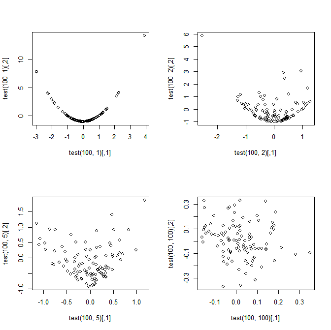
This doesn't prove anything, of course, but I always find doing simulations and plotting graphs to be very handy for making sense of theoretical results.

This is a particularly simple case. We generate $n$ random normal variates and compute $S_n$ and $T_n$; repeat $m$ times. Plotted are the graphs for $n = 1, 10, 100$ and $1000$. It's easy to see the dependence weakening as $n$ increases; at $n = 100$ the graph is almost indistinguishable from independence.

test <- function (m, n) 
{
    r <- matrix(rnorm(m * n), nrow = m)
    cbind(rowMeans(r), rowSums(r^2 - 1)/n)
}

par(mfrow=c(2,2))
plot(test(100, 1))
plot(test(100, 2))
plot(test(100, 5))
plot(test(100, 100))