Deletion residuals

Question

Please can you help me to solve this problem. It should be calculated by vectorization. The question is:

The i-th deletion residual $e_{(-i)}$ is defined as $e_{(-i)} = y_i - X^\top B_{(-i)}$
where $(X^\top)$ is the i-th row of the design matrix $X$ and $B_{(-i)}$ is a column vector of least square parameter estimates calculated without the i-th observation. Write some annotated R code to calculate the deletion residuals when the linear model $y_i = B_0 + B_1 X_i + B_2X_i^2 + E_i$
is fitted to the data in the file quadratic.txt. By drawing suitable plot, comment on the distribution of these deletion residuals.

---

Edit

I wrote some r codes , but it just gives me residual. I want to calculate deletion residual for i-th cases.

> quad<-read.table("quadratic.txt", header=T)
> quad

tha data is like this

x=(0.75078002, 0.70959645 ,0.07482854,0.60755927 ,0.55037327 ,0.55037327,   
0.35458257 ,0.21994714,0.66369585,0.12381099, 0.12381099,0.12381099,  
0.77869635,0.63917962) 

and

y=(18.715191,17.394049,-2.346149,5.528978,6.765831,6.324425,13.803874,  
15.007047,4.034973,12.383765,14.823395)

> quad.lm<-lm(y~x+I(x^2), data=quad)
> resid(quad.lm)
        1          2          3          4          5          6          7 
3.7933593  3.2646946 -4.9080046 -6.6589585 -4.3477835 -1.1856694  8.7046506 
        8          9         10         11 
1.7549092  0.6237708 -3.0781575  2.0371889 

Answer 1

This kind of jackknifing problem can be programmed straightforwardly, but that usually results in a tangle of for loops. Some linear algebraic manipulations go a long way in drastically reducing code length (if your computer's memory can handle it).

---

• Consider the original regression equation $$ Y_i= \boldsymbol{X}_i'\boldsymbol{\beta} + \varepsilon_i;\;i=1, \ldots, n $$ where $\boldsymbol{X}_i$ is a $k\times 1$ vector of regressors.You can write this more compactly as $$ \boldsymbol{Y} = \mathbf{X}\boldsymbol{\beta} + \boldsymbol{\varepsilon} $$

• Then the model that you want to estimate can be stacked up as $$ \begin{bmatrix} \boldsymbol{Y}^{(-1)} \\ \vdots \\ \boldsymbol{Y}^{(-n)} \\ \end{bmatrix} = \begin{bmatrix} \mathbf{X}^{(-1)} & & \\ & \ddots & \\ & & \mathbf{X}^{(-n)} \end{bmatrix} \underbrace{\begin{bmatrix} \boldsymbol{\beta}^{(-1)} \\ \vdots \\ \boldsymbol{\beta}^{(-n)} \\ \end{bmatrix}}_{\equiv \boldsymbol{\beta}^-} + \begin{bmatrix} \boldsymbol{\varepsilon}^{(-1)} \\ \vdots \\ \boldsymbol{\varepsilon}^{(-n)} \\ \end{bmatrix} $$ where $\boldsymbol{Y}^{(-i)} = [Y_1, \ldots, Y_{i-1}, Y_{i+1}, \ldots, Y_n]'$ is the $n-1 \times 1 $ vector with the $i$-th row (of $\boldsymbol{Y}$) deleted; and $\mathbf{X}^{(-i)} = [\boldsymbol{X}_1, \ldots, \boldsymbol{X}_{i-1}, \boldsymbol{X}_{i+1}, \ldots, \boldsymbol{X}_n]'$ is the $(n-1)\times k$ matrix with the $i$-th row (of $\mathbf{X}$) deleted. Note that the design matrix in this regression equation is block diagonal. Also, this is a very large system.

• Once $\widehat{\boldsymbol{\beta}}^-$ in the system above is estimated (by least squares), the residuals you want to estimate ($Y_i - \boldsymbol{X}_i'\widehat{\boldsymbol{\beta}}^{(-i)}$) can be had simply as $\boldsymbol{Y} - \mathrm{diag}(\mathbf{X}\mathrm{ivec}(\widehat{\boldsymbol{\beta}}^-))$, where the $\mathrm{diag}$ operator extracts the diagonal and $\mathrm{ivec}$ is the inverse of the $\mathrm{vec}$ operator which stacks the columns of the matrix.

---

R code

Here is some R code to show how this can be done. The only trick here is constructing the stacked, row-deleted matrices, and then you are left with one (very) large least squares problem to solve.

iN <- 50                # number of observations
iK <- 4                 # number of regressors (including constant)

mX <- matrix(rnorm(iN*iK), nrow = iN, ncol = iK)  # design matrix
vBeta <- c(1, 2, 3, 4)                            # coefficients
vY <- mX%*%vBeta + matrix(rnorm(iN))              # dependent variable
mXStacked <- (diag(iN)%x%mX)[-seq(from = 1, 
                                    to = iN*iN, by = iN+1), ]  # Stacked design matrix
vYStacked <- vec(vY%*%t(rep(1, iN)))[-seq(from = 1, 
                                            to = iN*iN, by = iN+1), ]   # Stacked outcomes
vBetaMinus <- solve(t(mXStacked)%*% mXStacked, 
                    t(mXStacked)%*%vYStacked)           # estimated coefficients
mBetaMinus <- matrix(vBetaMinus, nrow = iK, ncol = iN)
vResid <- vY - diag(mX%*%mBetaMinus)                  # required residuals

matplot(vResid, type = "l")           # plot the estimated residuals

Given dataset

The above R code can be easily adapted to the given dataset. Your outcome vector appears to be shorter than the regressor vector, so I have clipped off some of the latter.

vY <- as.matrix(c(18.715191,17.394049,-2.346149,5.528978,6.765831,6.324425,13.803874,  
   15.007047,4.034973,12.383765,14.823395))
x <- c(0.75078002, 0.70959645 ,0.07482854,0.60755927 ,0.55037327 ,0.55037327,   
   0.35458257 ,0.21994714,0.66369585,0.12381099, 0.12381099) 
mX <- as.matrix(cbind(constant = 1, x = x, x2 = x^2))
iN <- nrow(mX)
iK <- ncol(mX)
mXStacked <- (diag(iN)%x%mX)[-seq(from = 1, 
                                    to = iN*iN, by = iN+1), ]  # Stacked design matrix
vYStacked <- vec(vY%*%t(rep(1, iN)))[-seq(from = 1, 
                                            to = iN*iN, by = iN+1), ]   # Stacked outcomes
vBetaMinus <- solve(t(mXStacked)%*% mXStacked, 
                    t(mXStacked)%*%vYStacked)           # estimated coefficients
mBetaMinus <- matrix(vBetaMinus, nrow = iK, ncol = iN)
vResid <- vY - diag(mX%*%mBetaMinus)                  # required residuals

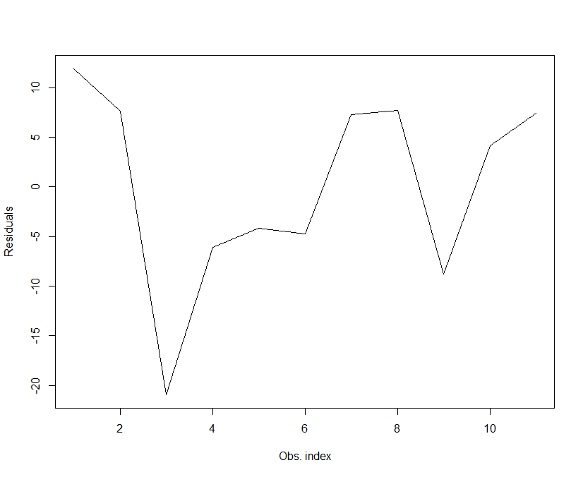
matplot(vResid, type = "l", xlab = "Obs. index", ylab = "Residuals")           # plot the estimated residuals

This produces the following picture.