how to find 10th, 50th, 90th percentile of a uniformly distributed data for all cases?

Question

Here are some key data to use for calculation:

1. initial population is 100, and average food consumption per person is 5lbs of rice each week
2. 1~2% of population dies off every month
3. 20~40 is added to population every month
4. average rice consumption per person increases by 0~2.5% weekly

Assumptions:

• assume all random variables are independent
• assume all variables are uniformly distributed across the given range.

Here is the question:

How is the food consumption growth of the population for the next 5 months in the 10th, 50th, and 90th percentile cases?

note:

this is a take home assessment that i cannot do. for personal growth, i'd like to learn how to do such problem. I feel like it'd be useful for IRL as well. i don't even know what to google to solve for this problem, hence i'm turning to this community for some suggestion/guidance/solution.

Thank you very much in advance.

Answer 1

This is a nice and neat simulation that I can demonstrate with R code. I would start off by defining the initial values:

population <- 100
consumption_rate <- 5

Next, we could define a few functions to vary the population parameters, as specified in the 3 steps:

## Take a uniform value in 0.01-0.02 as a percentage of our current population
death_rate <- function(population) {
  prop <- runif(1, 1, 2) / 100
  round(population * prop)
}
## Generate a random number births in range 20-40
birth_rate <- function() {
  round(runif(1, 20, 40))
}
## Generate an 0-2.5% increase in consumption rate
consumption_increase <- function(consumption_rate) {
  increase <- runif(1, 0, 2.5) / 100
  consumption_rate * (1 + increase)
}

The final step would be to run a number of simulations where we chain these simple functions together. The function replicate is very useful for situations like this.

simulations <- replicate(10000, {
    total_consumption <- 0
    for (i in 1:5) {
      population <- population - death_rate(population)
      population <- population + birth_rate()
      consumption_rate <- consumption_increase(consumption_rate)
      consumption_this_month <- population * consumption_rate
      total_consumption <- total_consumption + consumption_this_month
    }
    total_consumption
  }
)

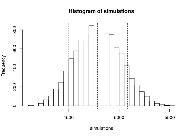
We now have total cumulative consumption measures from each of these 5 month simulations, and can easily visualise and calculate quantiles:

hist(simulations, breaks = "FD")
q <- quantile(simulations, c(0.1, 0.5, 0.9))
abline(v = q, lty = "dashed")

You'll no doubt notice that the results of the product of all of these uniformly distributed processes is actually (approximately) a normal distribution.

Note: the order in which actions happen (births, deaths, increase in consumption) in the simulation loop could have a strong effect on the outcome. This is something you would have to think about, I've just picked an arbitrary order.